Chapter 3 - Basic Geologic Principles & Maps |
|
3.1
Earth science is founded on basic principles that are useful for making many useful observations about the world around us. This chapter presents a mix of information that is essential (fundamental) to all following chapters. This chapter expands on the concepts focused on the solid earth (geology). We begin with a discussion on geologic time and the rock cycle — a graphic and conceptual model to illustrate common rocks and earth materials and the processes that form or change them, over time.
A Focus On Interpretation
Several basic geologic principles can be applied to resolving the order of events leading to the formation of rocks and landscape features. This section presents many basic concepts that are universal to all physical sciences. Geologists use geochronology — the study of the age of rocks, using both absolute dating methods and relative dating methods.
The second half of this chapter focuses on maps and the display of geographic and geologic information in two-dimensional and three-dimensional formats.
Geologic maps are essential components to resolving the geologic story (and history) of a region, and serve many useful purposes for society including uses in urban planning, agriculture, health and public safety, mineral resource management, water resources, and much more.
|
Click on thumbnail images for a larger view. |
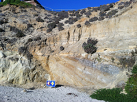
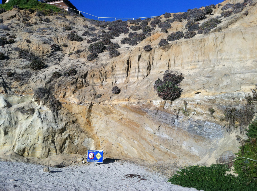
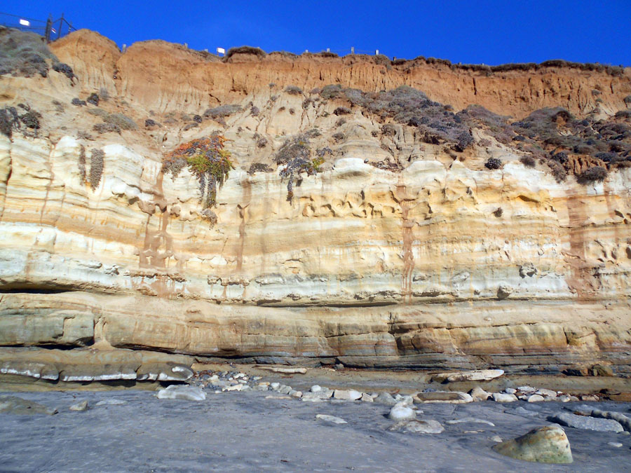
Fig. 3-1. Layered sedimentary rocks in a sea cliff in Encinitas, CA showing an angular unconformity (evidence of a gap in the geologic record). |
3.2
Basic Geologic Principles For Interpreting Landscape Forming Processes
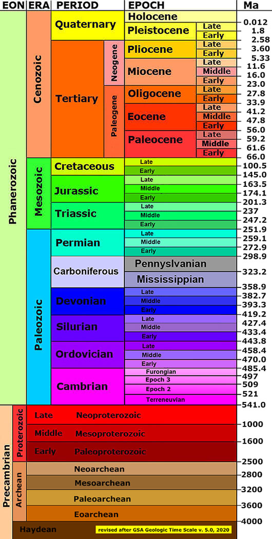
The surface of the Earth is shaped by processes moving materials underground and by processes occurring on the surface under the influence of atmospheric, hydrologic, and oceanographic processes. The logical place to start discussion is to examine the material below our feet. Perhaps most fundamental to understanding the geologic origin of landscapes and earth materials is the vastness of geologic time. It took centuries for the scientific community to compile information about the age of different regions in the planet through the study of rocks, the fossils they contain, and the chronology of events in Earth's history (such as the formation of mountain ranges, changes in coastlines, and the evolution of life). One of the products of this collective investigation over time is the geologic time scale (Figure 3-2). The time scale links measures of time (on the scale of periods ranging from thousands, millions, to billions of years) to established names for those time periods used in publications (reports and maps). The geologic time scale has been continuous refined as new data is collected. (See section 1.10 in Chapter 1 for a discussion on geologic time.)
What Is Bedrock?
Bedrock is the solid rock that occurs beneath soil or alluvium (unconsolidated sediments) that coved the surface of the land in most locations. In some places the bedrock is exposed as rocky outcrops scattered across the landscape, particularly in mountainous areas or along stream canyons. The term outcrop is used to describe a location where bedrock is exposed (or crops out).
Why do landscapes in different areas have unique characteristics? Its all about the bedrock and its history!
Landscapes change from one region to the next because of the composition and character of bedrock changes from place to place.
Geologists attempt to unravel geologic history by studying the geometry of outcrops in an area. Subtle characteristics of undisturbed landscapes often reveal the location of faults, ore deposits, sources of groundwater, and many other features of geologic interest.
|
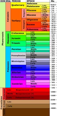 Fig. 3-2. Geologic Time Scale Fig. 3-2. Geologic Time Scale |
3.3
The Rock Cycle and Rock Classification (revisited)
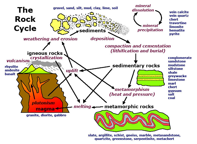
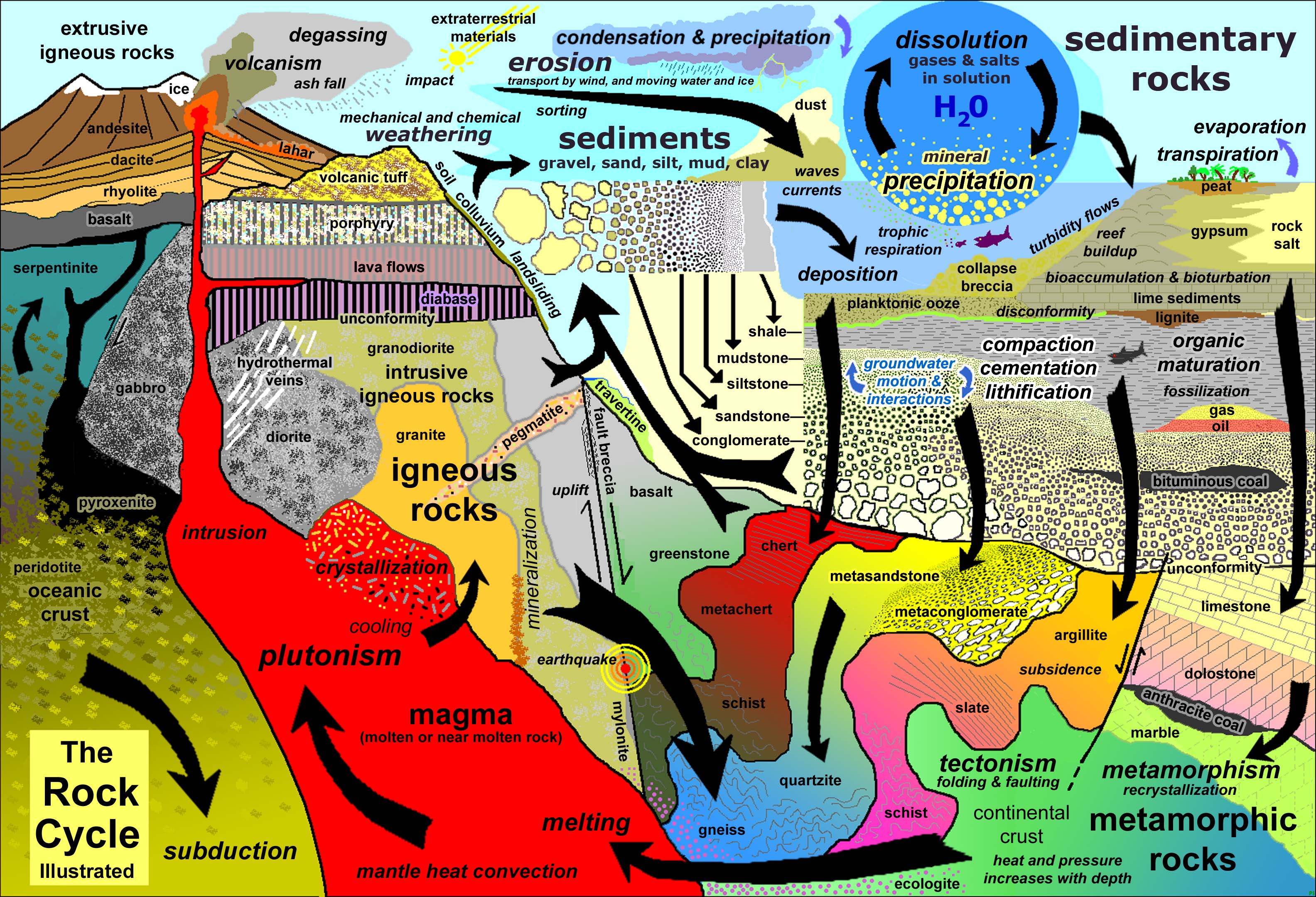
Charles Lyell (1797-1875) compiled the first geology textbook entitled "Principles of Geology" in which he promoted concepts of the "rock cycle" (Figure 3-3). The rock cycle illustrates the series of events in which a rock of one type is converted to one or more other types, and then possibly back to the original type. The rock cycle is a graphic and conceptual model to illustrate common kinds of rocks and earth materials and the processes that form or change them over time. Figure 3-4 also illustrates the rock cycle—but includes more detail about both rocks and earth materials, and selected geologic features associated with geologic processes. Be sure to examine the arrows on the diagrams! Pathways to rock origins may go several routes—rocks of any kind can be changed in different ways into a variety of other rocks types. It is important to note that tectonic forces within the Earth are responsible for many of the changes to rocks and surface features on the landscape. Tectonic forces are responsible for the gradual uplift of mountain ranges, both on land and on the seafloor, as well as creating basins that flood with lakes or seawater, and fill in with sediments (Figure 3-5).
There are 4 classes of rocks and earth materials: igneous rocks, sediments (which are not rocks), sedimentary rocks, and metamorphic rocks.
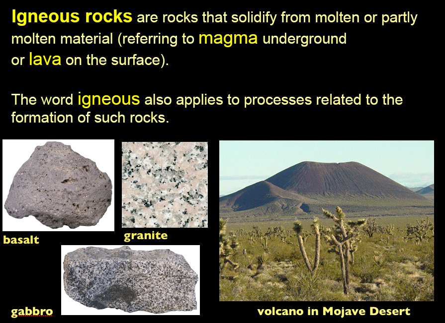
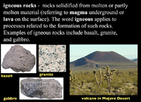
Igneous rocks are rocks formed from the cooling and crystallization of molten materials (Figure 3-6). The word igneous applies to any rock or mineral that solidified from molten or partly molten material (referring to magma underground or lava on the surface). The word igneous also applies to the processes related to the formation of such rocks. Igneous rocks includes intrusive rocks (rocks that cooled below the surface) and volcanic rocks formed on the Earth's surface by volcanism. Igneous rocks also form from melting associated with extraterrestrial impacts. Examples of igneous rocks include granite, gabbro, and basalt. Rocks of igneous origin are discussed in Chapter 9.
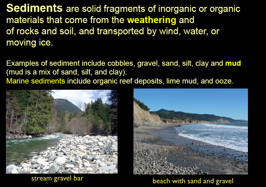
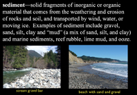
Sediments are solid fragments of inorganic or organic material that come from the weathering of rock and soil erosion, and are carried and deposited by wind, water, or ice (Figure 3-7). Sediments may be made up of rock fragments ranging is size from boulders down to microscopic particles, and may contain organic matter. Examples of sediment include gravel, sand, silt, clay, mud (mix of sand, silt, and clay), soil, lime mud, and ooze. Sediments are not rocks, but they may become rocks through heating, compaction, and cementation. Sediments are discussed in Chapter 10.
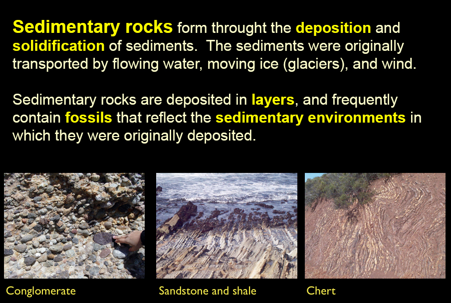
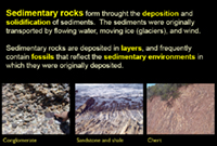
Sedimentary rocks are rocks that have formed over time through the deposition and solidification of sediment, especially sediment transported by water (rivers, lakes, and oceans), ice ( glaciers), and wind (Figure 3-8). Sedimentary rocks are often deposited in layers, and frequently contain fossils. Sedimentary rocks are often deposited in layers, and frequently contain fossils. Examples of sedimentary rocks include shale, sandstone, conglomerate, limestone, and chert. Sedimentary rocks are discussed in Chapter 11.
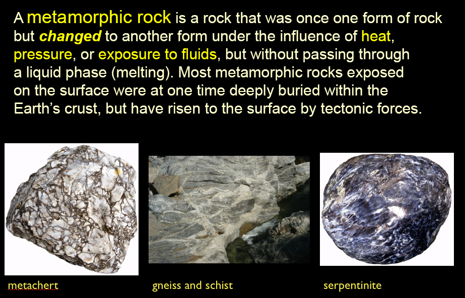
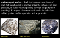
Metamorphic rocks are rocks that was once one form of rock but has changed to another under the influence of heat, pressure, or fluids without passing through a liquid phase (melting) (Figure 3-9). Examples of metamorphic rocks include slate, schist, gneiss, marble, quartzite, and serpentinite. Metamorphic rocks are discussed in Chapter 12.
These rock cycle diagrams illustrate how earth materials form and change over time. Both products (rocks and sediments) and processes (such as melting, cooling, erosion, and deposition) are illustrated. The passage of geologic time is an essential component, although some processes are much faster than others. Note that all these types of processes are taking place simultaneously, but at different locations on and within the planet. |

Fig. 3-3. The Rock Cycle: processes are in purple; products are in black and blue. |
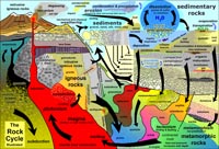
Fig. 3-4. Rock Cycle Illustrated. This version of the rock cycle shows more detail in graphic form. It is good to compare the two diagrams.
|
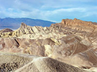
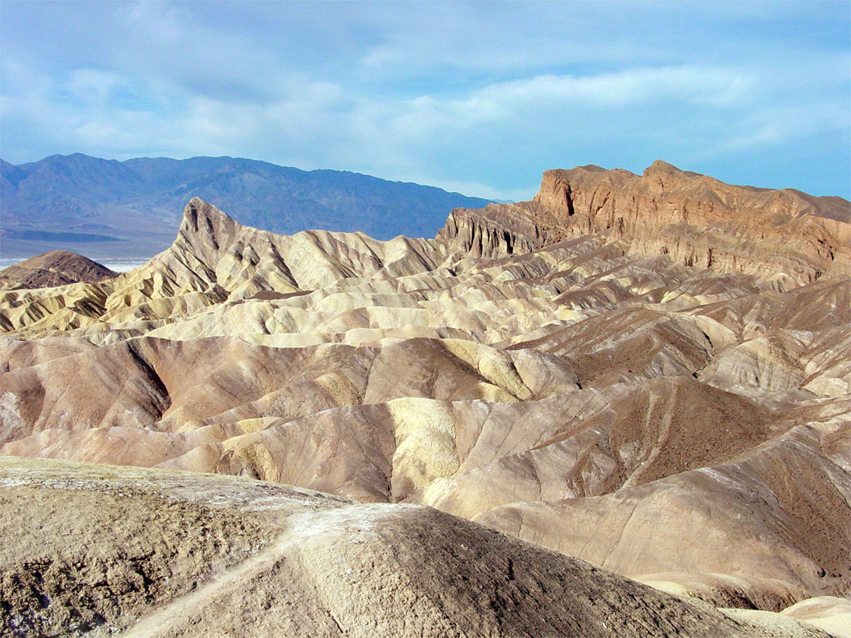
Fig. 3-5. The rock cycle includes examination of tectonics, forces that raise or lower the surface of the land and seafloor. Tectonic forces are responsible for creating mountain ranges and basins that fill with sediments. This view show the dynamic (changing) landscape of Death Valley, California. |
 |
 |
 |
 |
| Fig. 3-6. Igneous rocks |
Fig. 3-7. Sediments |
Fig. 3-8. Sedimentary rocks |
Fig. 3-9. Metamorphic rocks |
|
3.4
Preview of Selected Concepts Related To the Rock Cycle |
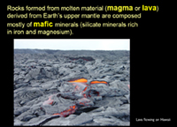 |
Fig. 3-10. Igneous rocks from the cooling of molten material (magma, lava) and are rich in silicate minerals. Molten material derived from deep in the Earth's mantle is typically enriched in iron- and magnesium-rich silicate minerals (and the rocks they form, these are called mafic or ultramafic). In contrast, magma and lava associated with continental crustal regions are enriched in felsic silicate minerals rich in silicon and aluminum (mostly feldspars) (The importance of felsic and mafic minerals are introduced below). This contrast between mafic and felsic materials is important to discussion about plate tectonics in Chapter 5. |
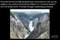 |
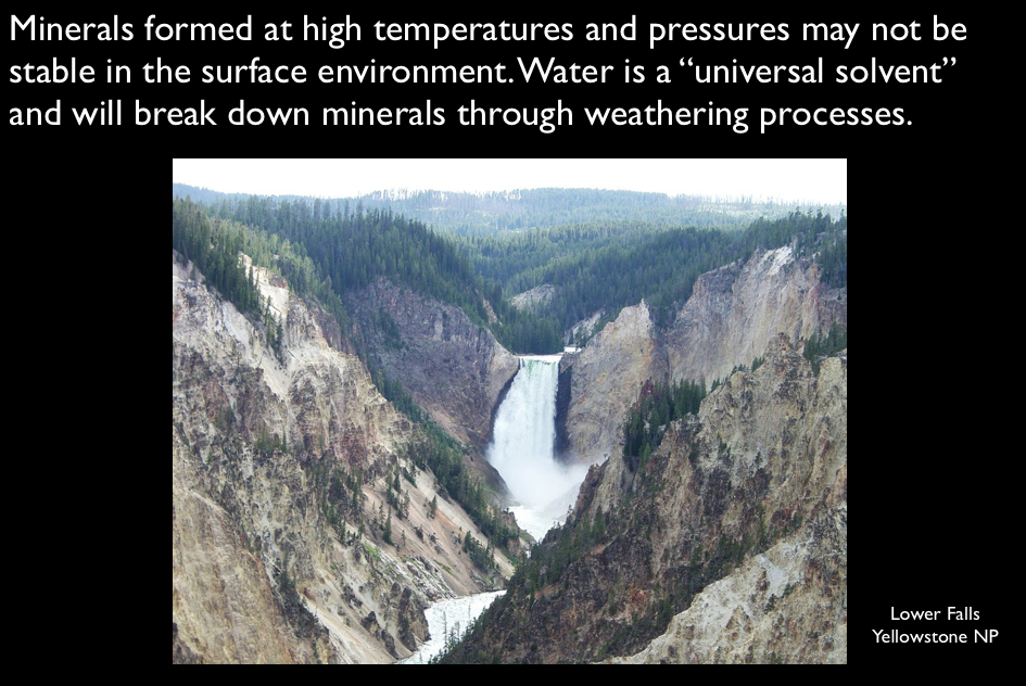
Fig. 3-11. Weathering of rocks and minerals: Water (H2O) occurs in rocks within the earth and is a primary chemical agent on the earth surface. Water is called the "universal solvent," dissolving and transporting material in solution, altering the chemical composition of mineral, and transporting sediment (erosion and deposition). Not all rocks and minerals behave similarly when subjected to weathering and erosion. Hard and durable minerals like quartz tend to resist weathering and erosion, and therefore can be carried long distances carried as sediments by flowing water or wind. |
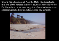 |
Fig. 3-12. Durability of quartz: Quartz an extremely abundant mineral in the Earth's crust. Quartz is also an extremely durable mineral (with a Mohs hardness of 7.0). As quartz-rich rocks weather and erode, minerals other than quartz tend to break down or decay into fine clay, whereas quartz grains tend to endure the abrasive processes while being transported by streams or battered by wave action on beaches. The finer clay materials get carried away by currents (water or wind). In contrast, the larger, more durable quartz grains become concentrated in the form of quartz-rich sand found on beaches and in desert sand dune fields. |
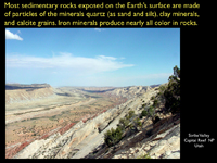 |
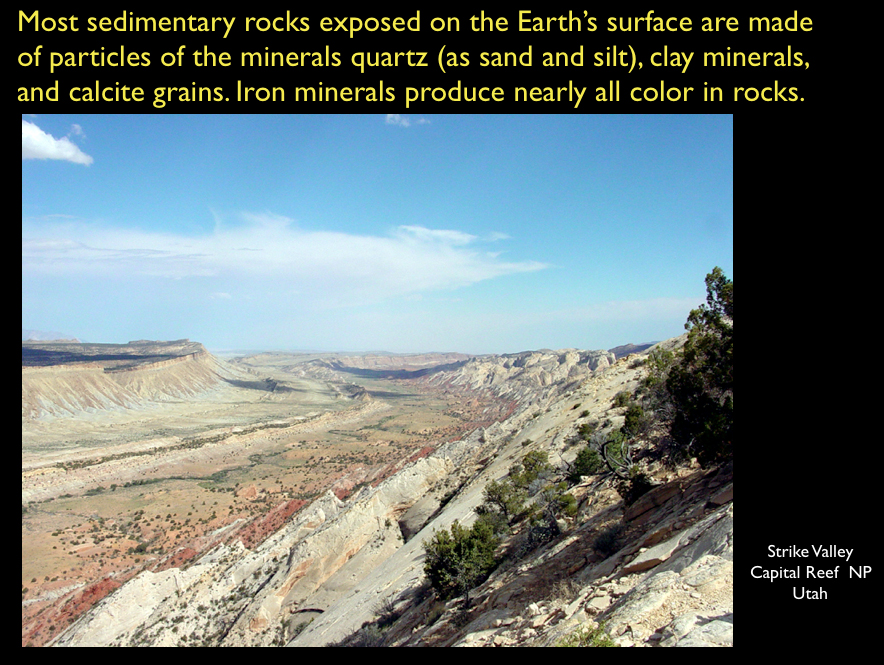
Fig. 3-13. Minerals in sedimentary rocks: Most sedimentary rocks are enriched in the minerals quartz, calcite, and some iron and clay minerals. Minerals with high hardness and low solubility are transported by erosion and deposited in sedimentary basins. Typically soft minerals that are highly soluble are dissolved and carried by surface and groundwater where most contributes to the saltiness of seawater. However, dissolved components in water can precipitate to form mineral cements, including like calcite (CaCO3), iron-rich minerals (hematite and limonite), and silica (quartz). The iron-mineral content in rocks are mostly responsible for the earth-tone colors they display. |
 |
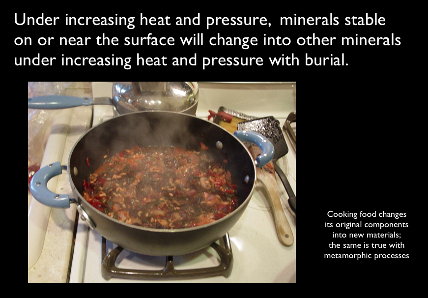
Fig. 3-14. Metamorphic processes cause changes in the mineral composition in rocks: Changes in heat, pressure, and exposure to fluids, over time, will change the mineral composition of earth materials, such as converting sediments into sedimentary rocks, and changing sedimentary and igneous rocks into metamorphic rocks. Conversely, exposing rocks to fluids—water and air at or near the surface—help to degrade rocks to form many kind into sediments. |
|
3.5
What is a rock formation?
Geologists who study and map the location of rocks in a region will assign them names and will described them by their composition and their geologic ages (if possible). A rock formation is a rock unit that is distinctive enough in appearance that a geologist can distinguish it from other surrounding rock layers. A named rock formation must also be thick enough and extensive enough to plot on a geologic map. Rock formations and geologic maps are a discussed in more detail below. Typically rock formations are named after a geographic feature or area associated with where a rock formation is exposed. for instance, the Kaibab Formation is named after the Kaibab Plateau where it crops out extensively. The name of the rock formation may also contain the name of it's dominant rock type, such as the Torrey Pines Sandstone Formation, a massive sandstone deposit of Eocene age that crops out in the sea cliffs at Torrey Pines State Beach Preserve in San Diego County, California.
Layered Versus Non-Layered Rocks
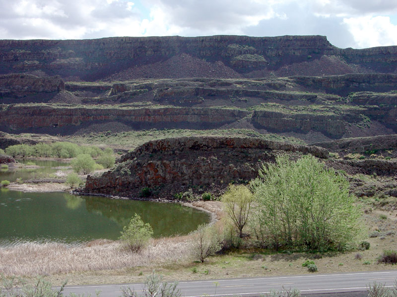
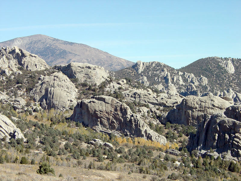
Large bodies of rocks typically display recognizable characteristics, most notable are characteristics of rock layers—called strata. Strata are layered rocks that are typically formed when an accumulation of rock material is deposited in a setting, then as time passes more layers accumulate on top. If cut and exposed by erosion or faulting, the layers appear as a series of beds. (A single bed is called a stratum). Rocks that display layering are called stratified; rocks that do not display obvious layering are called unstratified (Figures 3-15 to 3-18).
Some rocks are layered (or stratified), others are not. Sedimentary rocks and some volcanic deposits (lava flows and air-fall volcanic ash deposits) are examples of commonly stratified rocks. Examples of rocks that are unstratified are igneous rocks (like granite) that cooled and crystallized deep underground and did not develop layers. Also, rocks that have experienced extensive metamorphism and remelting may no longer preserve stratification. (As always, in geology, and science in general, there are sometimes exceptions to these rules!) |
3.6
Sedimentary rock formations display features that reveal information about the environments where they formed.
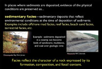
The term sedimentary facies is used to describe or interpret the origin of sedimentary deposits that reflect environmental conditions that existed at the time the sediments were deposited. Examples include: offshore mud facies, reef facies, beach sand facies, terrestrial swamp facies, etc. Facies reflect the character of a rock expressed by its formation, composition, and fossil content associated with the physical conditions at the time that they formed (Figure 3-13).
Sedimentary facies preserved in rock formations reveal much information about earth history, including how climates and geography have changed. They can reveal information about the timing of the formation of nearby mountain ranges, the movement of faults (associated with earthquakes), eruption of volcanoes, and the shifting of shorelines over time. |
 |
| Fig. 3-19. Sedimentary facies reveal information about past environmental conditions. |
3.7
Basic Geologic Principles
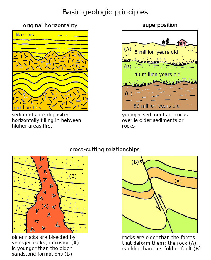
In 1669, Nicolas Steno first proposed several basic geologic principles that were later embellished by notable Scottish geologists, James Hutton and Charles Lyell (introduced in Chapter 1). These basic principles are easily observed in geologic outcrops bearing layered rocks (strata), but have value for any number of scientific and technical applications beyond geology. Figure 3-20 illustrates basic geologic principles for Steno's three laws that are used in resolving the relative age of rocks and the order in which they formed or as geologic events occurred.
Steno's three laws are as follows:
Law of Original Horizontality—this law states that most sediments, when originally deposited, were laid down horizontally. However, many layered rocks are no longer horizontal—faulting and tectonic forces, and volcanic activity can deform rock layers
Law of Superposition—this law states that in any undisturbed sequence of rocks deposited in layers, the youngest layer is on top and the oldest on bottom, each layer being younger than the one beneath it and older than the one above it.
Law of Cross-Cutting Relationships—this law states that a body of igneous rock (an intrusion), a fault, or other geologic feature must be younger than any rock across which it cuts through.
Note that the boxes in Figure 3-19 illustrate vertical cross sections of what may exist below the surface. Cross sections are discussed more below. |
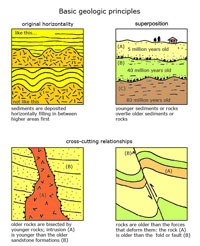
Fig. 3-20. Basic geologic principles illustrated. The four boxes represent vertical profiles below the ground surface, or a view such as may appear in a cliff on the side of a mountain or canyon. |
3.8
Unconformities: Gaps In the Geologic Record
Following on the Law of Original Horizontality and Law of Superposition, both Hutton and Lyell recognized erosional boundaries preserved between rock layers
representing gaps in the geologic record. They named these gaps unconformities (examples in Figure 3-21). An unconformity is a surface between successive strata that represents a missing interval in the geologic record of time. Unconformities show evidence that the Earth's surface may have been exposed to erosion for periods of time. Unconformities are produced either by an interruption in deposition or by the erosion of per-existing strata followed by renewed deposition. Note that unconformities can be complex. For example, may erosion may be taking place in one location in geologic time, where nearby or elsewhere sediments may have continued to be deposited and preserved. As a result, an unconformity in one location may span a different about of time in another location.
Several types of unconformity boundaries are recognized:
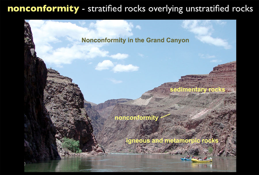
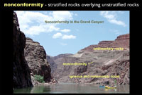
- nonconformity—an unconformity between sedimentary rocks and metamorphic or igneous rocks when the sedimentary rock lies above and was deposited on the pre-existing and eroded metamorphic or igneous rock
.
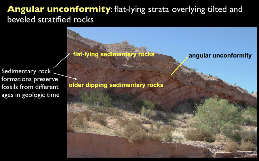
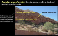
- angular unconformity—an unconformity where horizontally parallel strata of sedimentary rock are deposited on tilted and eroded layers, producing an angular discordance with the overlying horizontal layers
.
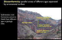
- disconformity—an unconformity between parallel layers of sedimentary rocks which represents a period of erosion or non-deposition.
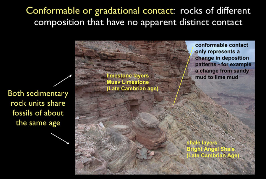
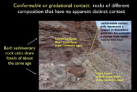
- conformable boundary—an arrangement where layers of sedimentary strata are parallel, but there is little apparent erosion and the boundary between two rock layer surfaces resemble a simple bedding plane. There is typically little evidence to support a significant passage of time occurred at a conformable boundary.
|
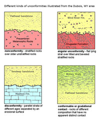
Fig. 3-21. Types of unconformities (boundaries between layered rocks representing "gaps" in the geologic record in a locality). The four boxes represent vertical profiles below the ground surface, or a view such as may appear in a cliff on the side of a mountain or canyon. |
| Examples of unconformities and conformable boundaries in the Grand Canyon of Arizona |
 |
 |
 |
 |
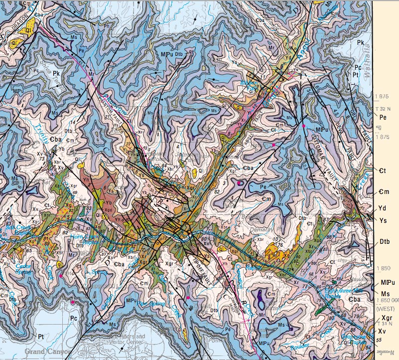
| Fig. 3-22. Nonconformity in the Grand Canyon (known as the "Great Unconformity") between Precambrian-age metamorphic rocks and overlying Cambrian-age sedimentary rocks. |
Fig. 3-23. Disconformities between layers in the Grand Canyon. Disconformities occur between sedimentary rock formations of different ages and represent gaps of time spanning millions of years. |
Fig. 3-24. An angular unconformity occurs between sedimentary rocks of different ages. Uplift and erosion of a mountainous landscape occurred before the overlying sediments were deposited. |
Fig. 3-25. Conformable or gradational contact between sedimentary layers. This type of boundary only reflect a change in how sediments were depositied—not necessarily representing a long gap in time. |
|
3.9
How Do Unconformities Form?
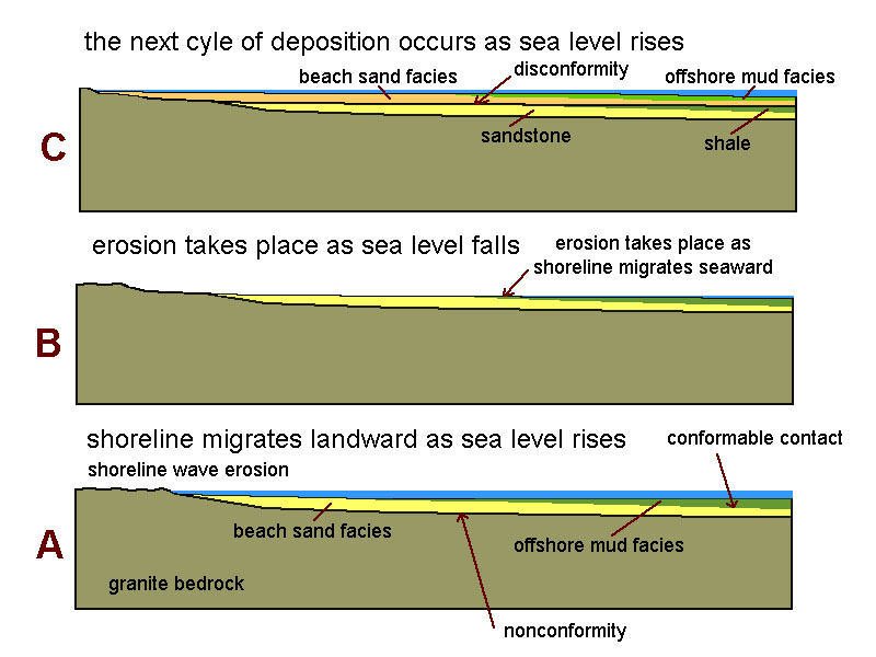
Unconformities are caused by relative changes in sea level over time. Wave erosion wears away materials exposed along coastlines, scouring surfaces smooth. On scales of thousands to millions of years, shorelines may move across entire regions. Erosion strips away materials exposed to waves and currents. New (younger) material can be deposited on the scoured surface. Shallow seas may flood in and then withdrawal repeatedly. Long-lasting transgressions can erode away entire mountain ranges with enough time.
A transgression occurs when a shoreline migrates landward as sea level (or lake level) rises.
A regression occurs when a shoreline migrates seaward as sea level (or lake level) falls (Figure 3-26).
Sea level changes may be caused by region uplift or global changes in sea level, such at the formation or melting of continental glaciers. Whatever the cause of sea level change, when sea level falls, sediments are eroded from exposed land. When sea level rises, sediments are typically deposited in quiet water settings, such as on shallow continental shelves or in low, swampy areas on coastal plains.
Some unconformities represent great gaps in time. For example, the Great Unconformity in the lower Grand Canyon illustrates where a great mountain range existed in the region during Precambrian before erosion completely stripped the landscape away back down, eventually allowing seas to flood over the region again in Cambrian time. The "gap in the geologic record" in some locations along the Great Unconformity represents billions of years (see Figure 3-21).
|
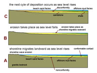
Figure 3-26. Unconformities can form by the rise and fall of sea level. Erosion strips away materials exposed to waves and currents. A rise in sea level causes a transgression which creates space underwater for sediments to be deposited. New (younger) material is deposited on the scoured surface. When sea level falls it causes a regression, and sediments are not deposited or are eroded away. |
3.10
How are the ages of rocks determined?
Geochronology is the branch of earth sciences concerned with determining the age of earth materials and events through geologic time.
How do geoscientists determine the age of rocks or fossils? How do they figure out how long ago and in what order did geologic processes or events take place? For instance how do they know how often a volcano erupts or how often earthquakes take place? Geologists now have many ways to determine the age of materials using relative dating and absolute dating methods.
Relative Dating
Relative dating is the science of determining the relative order of past events, without necessarily determining their absolute age (see below). Relative dating involved the study of fossils and the correlation or comparison of fossils of similar ages but from different regions where their age is known. Microfossils derived from sediments and cores from wells help in the subsurface exploration for oil and gas.
When studying an area where layered rocks are exposed, the Law of Original Horizontality dictates that the sedimentary layers were originally deposited as flat layers. The Law of Superposition dictates that if a series of rock layers are exposed, the oldest are on the bottom of the stack. That is true, unless the sequence of rock layers have been disturbed by some later geologic even. It that case, the Law of Cross-Cutting Relationships dictates that the rocks will be older than the forces that later changed them. Examples of forces that change landscapes include movement of faults, or the tectonic folding of rock layers, or an intrusion of igneous material, such as the formation of a volcano.
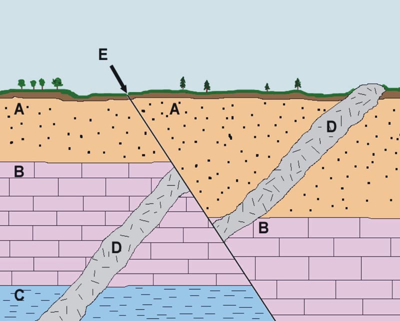
Example! Use these rules to interpret this general vertical cross section of a landscape (Figure 3-27). The diagram could represent a road cut along a highway or a wall on the side of a canyon. The Law of Original Horizontality and Law of Superposition suggest that layer C (layers of shale) was deposited before layer B (beds of limestone), which was deposited before layer A (beds of sandstone). The Law of Cross-Cutting Relationships dictates that next thing to happen was that feature D (an igneous intrusion) cut across the sedimentary layers. After that a fault (feature E) broke through all the older materials. The final thing to happen was erosion of the landscape down to partially expose some of the features on the surface. Note also that the boundaries between layers C and B, and A and B may represent unconformities (possible gaps in time).
Relative dating only can be used to sort the exposed visible features in the order that they formed (example in Figure 3-28).
Fossils and Relative Dating
Sedimentary rock layers of different ages often look very similar. Conversely, sedimentary rock layers of similar ages may appear very different in other locations. Sometimes fossils preserved in sedimentary layers are very useful for correlating rock layers from one area or region to another. Paleontologists have extensively studied fossil found in sedimentary rock formation of all geologic ages around the world. Certain "index fossils" are both abundant and widely distributed through sedimentary rocks of relatively limited geologic time ranges.
Unfortunately, many rocks formation do not contain fossils, or the fossils they may contain are very rare or poorly preserved. Metamorphic and igneous rocks do not contain fossils. In many cases, the exact age of each of the rock units is unknown until it can be confirmed by other means involving absolute dating methods (discussed below). |
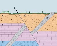
Fig. 3-27. Applying basic geologic principles: Laws of Original Horizontality, Superposition, and Cross-Cutting Relationships explain the order of this diagram with the order of formation: rock units C, B, A, D, then E (followed by surface erosion).
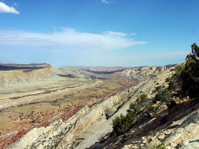
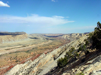 Fig. 3-28. Rock layers like these in Utah record information about 100 million years of Earth history exposed in the region. These rocks were originally deposited horizontally but then were later folded upward: oldest rocks on the right; youngest on exposed on the mesa top on the left. Fig. 3-28. Rock layers like these in Utah record information about 100 million years of Earth history exposed in the region. These rocks were originally deposited horizontally but then were later folded upward: oldest rocks on the right; youngest on exposed on the mesa top on the left. |
3.11

Fig. 3-29. Relative Dating Exercise #1. Tracks left in the mud along a river bank include a bear, bird, deer, dog, bobcat, and human (and blood). What happened, and in what order? |
Try Relative Dating (sort out the visually available clues in a map view).
The basic geologic principles have many applications to interpreting the order of events on many scales, ranging from very large (like the Grand Canyon or the geologic history of parts of the Rocky Mountains), to small scale, like interpreting the order of footprints along a lake shore (as illustrated in this exercise).
Geologists use basic geologic principles to study geology map (as illustrated below), and use them to unravel the complex history of an area, such as planning tunnels in large underground mining operations, or for exploring for oil and gas, and deep-water resources.
Try interpreting the order of events in the map-view diagrams involving animal trackways (Figures 3-29 and 3-30). Notice that some tracks overly (are superimposed) on other tracks. Sometimes things aren't as clear as they seem, but inferences can be made.
Basic geologic principles are used to interpret the geologic history of an area. See examples in Figures 3-31 to 3-34.
|
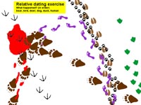
Fig. 3-30. Relative Dating Exercise #2. Tracks left in the mud along a river bank include a bear, bird, deer, bobcat, duck, and human. Can you figure out the chronology of events in this nature scene? |
3.12
Examples of how the basic geologic principles can be applied to relative dating on rock outcrops. |
 |
 |
 |
 |
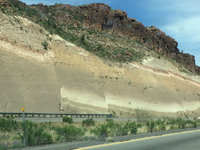
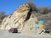
| Fig. 3-31. Minor faults cut though layers of volcanic ash beds and sedimentary rocks, exposed along I-40 near Kingman, AZ. |
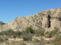
Fig. 3-32. Folded layers of sedimentary rocks exposed near the San Andreas Fault in Box Canyon near Mecca, CA. |
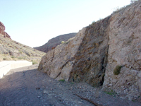
Fig. 3-33. A fault cuts trough sedimentary rocks along Arroyo Seco Canyon in the Santa Lucia Range in Monterey County, CA. |
Fig. 3-34. A basalt igneous intrusion cuts through older volcanic rocks in Lake Mead National Recreation Area, NV. |
|
In Figure 3-31, the Laws of Original Horizontality and Superposition show a series of sedimentary layers and volcanic ash bed deposited from oldest (on the bottom) to a lava flow (on the top of the cliff). The Law of Cross-Cutting Relationships shows that the layers were offset by faulting after they were deposited as layers.
In Figure 3-32. the Laws of Original Horizontality and Superposition indicate that this series of sedimentary layers were deposited horizontally before tectonic forces pushed up these layers located near to the San Andreas Fault. Therefore, the San Andreas Fault must be younger than the sedimentary layers.
In Figure 3-33, the Law of Cross-Cutting Relationships suggests that the fault in the picture is younger than the sedimentary rock formation on either side of the fault. However, the age of the two rock formation on either side would have to be determined by some other means (such as by the fossils they may contain).
In Figure 3-34, the Law of Cross-Cutting Relationships suggest that the dark, basalt igneous dike is younger than the pink volcanic rocks on either side, however, the exact age of the volcanic rocks would have to be determined by other means. |
3.13
Cross Sections
Cross sections are important tools for relative dating!
A geological cross-section is a graphic representation of the intersection of the geological features in the subsurface with a vertical plane. Where the vertical plane intersects the surface is typically shown as a line on a map. Like geologic maps, cross sections show different types of rocks, their structure, and the geometric relationship between them are represented. Note that geologic cross sections are made by using available mappable features found on the surface or interpreted from data about the subsurface. Natural cross sectional views are sometimes possible along canyon high walls or along steep mountain range front (Figure 3-35). How most subsurface data derive or imaged through geophysical methods, such as by seismic data (by earthquakes or man-made explosions), by measurements of gravity, magnetism, electrical resistivity, or information derived from wells such as core sample, radiation measurements, or other geophysical methods.
|
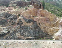
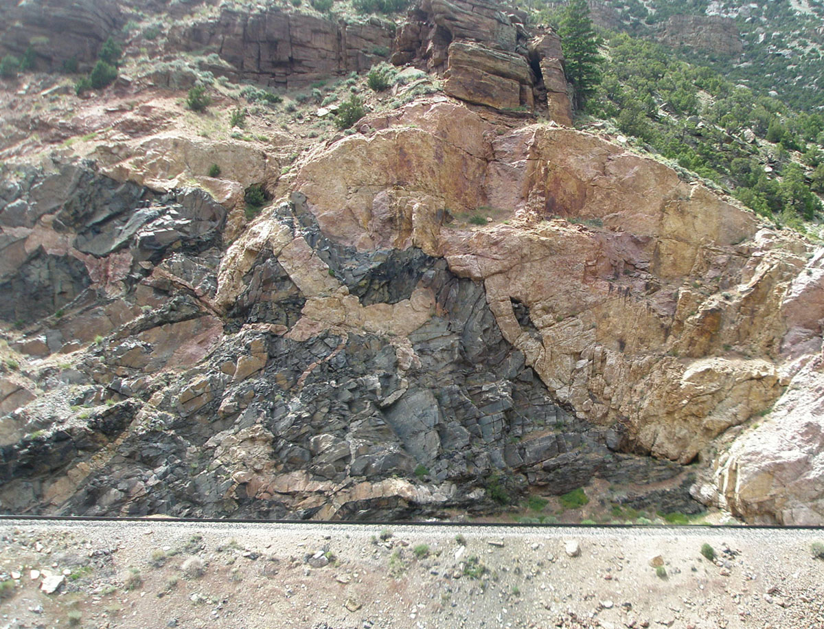
Fig. 3-35. A wall of rocks exposed in a cliff illustrate the vertical view illustrated by a cross section. This cliff shows igneous intrusions exposed in Wind River Canyon, Wyoming. |
3.14
Geophysical Methods Used To Make Cross Sections
Geologists have a variety of geophysical methods to collecting information about geologic features underneath the surface. For example, geologists use use sound (shock waves produced by explosives or machines making sounds to penetrate the ground). Other geophysical methods collect measurements using electricity and radar to penetrate the ground,
and measurements of variations in Earth's gravity and magnetism. In addition, geologists use data from wells drilled in an area to add information to cross sections.
Seismic Reflection Techniques Produce Cross Sections Used For Subsurface Exploration
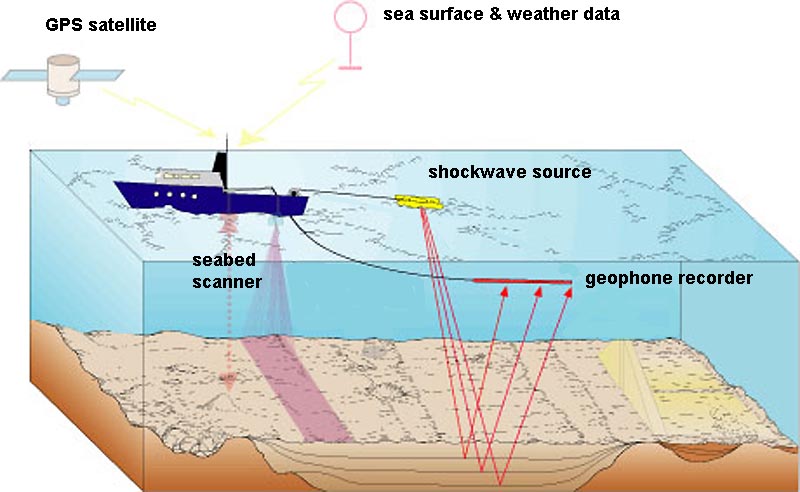
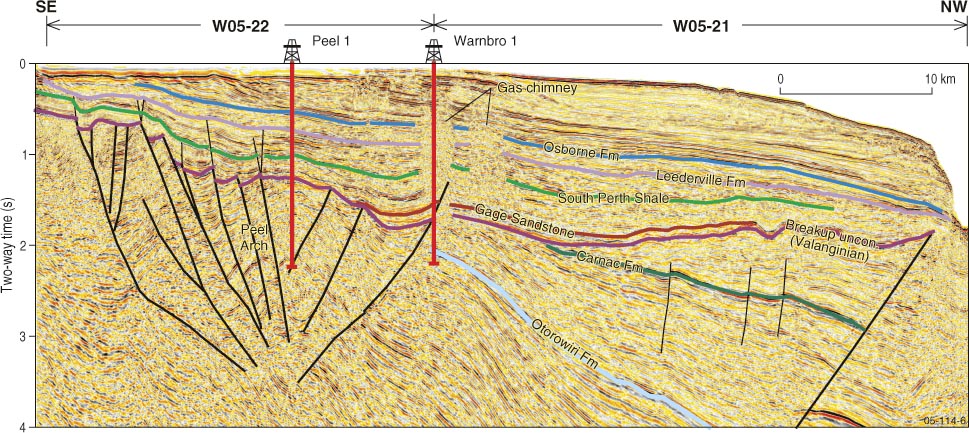
Seabed exploration produces cross-sectional seismic profiles, raw data that are converted to cross-section diagrams (Figure 3-36). Modern systems produce views that are in three dimensions.
Geologists study cross sections created by geophysical exploration methods. Figure 3-37 is an example of a seismic profile showing the location of exploratory wells.
|

Fig. 3-36. A marine seismic reflection profile expedition.
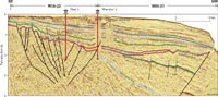 Fig. 3-37. A seismic reflection profile data is a cross section. Fig. 3-37. A seismic reflection profile data is a cross section. |
3.15
Relative Dating Using Cross Sections - Examples |
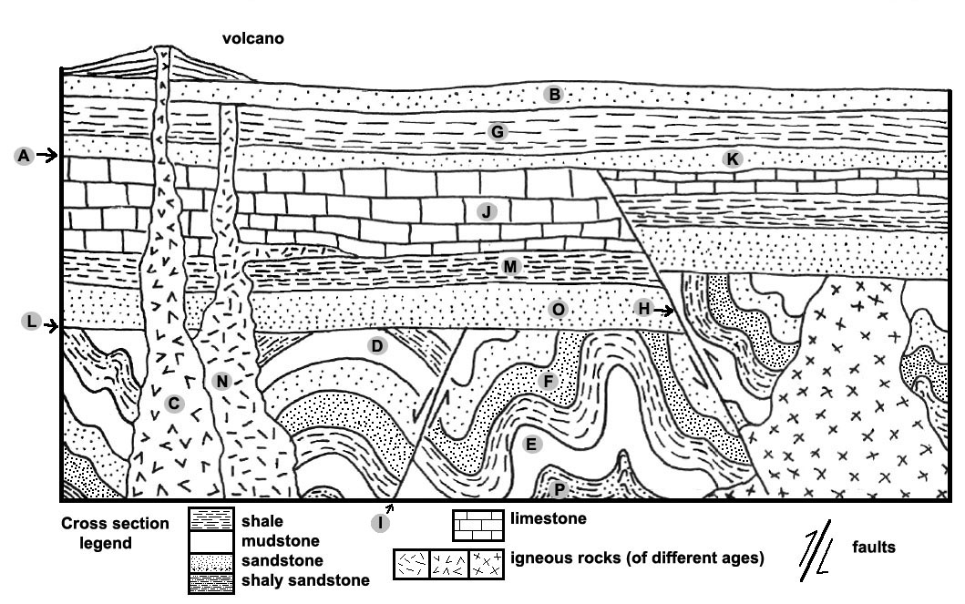
Figure 3-38 illustrates a cross section of a hypothetical landscape with an active volcano. Beneath the surface in this landscape are a mix of layered and non-layered rocks. Letters correspond to different features including a fault, unconformities, and the active magma chamber feeding lava to the volcano erupting on the surface. Examine the cross section to see the chronology of the formation of geologic features, from oldest to youngest represented by letters A to Q. [Be sure to review Figures 3-19 and 3-21, and open the larger view of Figure 3-38 while you review the information below.]
- Letter A represents ancient non-stratified rocks (possibly a mix of metamorphic and igneous rocks). These ancient rocks may have been an ancient mountain range that later wore down by erosion over time.
- Letter B represent a unconformity (an erosional gap in time) between the ancient rocks below and layer C, a layered sedimentary bed on of the older rocks (A). (The letter B is technically a nonconformity between stratified and non-stratified rocks).
- Sedimentary layers D and E were deposited (originally horizontal beds) on top of layer C.
- Letter F point to the unconformity that is actually younger than the unconformity at letter B! This unconformity represents a period of uplift and erosion before sedimentary layer G was deposited. This unconformity is a nonconformity or an angular unconformity depending where you examine it.
- Sedimentary layers G, H, I, J, and K were deposited in that order, following the Laws of Superposition and Original Horizontality.
- Another period of uplift occurred. During this time, a fault formed (Letter L). In addition layers G, H, I, J, and K were gently folded (warped) upward by renewed tectonic forces.
- Letter M represents another unconformity. This unconformity beneath layer N tells us that the fault (L) formed before sedimentary layer N was deposited on the eroded surface and younger than layer K. Note! Without more information we can only know that the fault (L) is younger than layer I but is younger than layer N.
- Sedimentary layer O horizontally rests on top of layer N.
- Finally, igneous activity produced volcano (P). Molten material is still flowing from the magma chamber (Q) to produce the active eruption on the volcano.
|
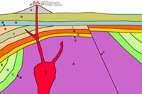
Fig. 3-38. A hypothetical cross section showing layers beneath a landscape with an active volcano in a region where mountain building has occurred in the ancient past.
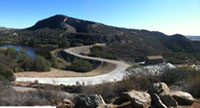
Fig. 3-39. The region around the extinct Calavera Hills Volcano in Carlsbad, California (San Diego County) has a similar geologic history as illustrated in Figure 3-38.
|
3.16
When working with cross sections is is often easiest to start from the "top" (youngest rocks) and work backwards in time to the "bottom" (oldest rocks). Then, work things out in reverse older to tell the geologic history of a region. Be sure to examine the geologic time scale to understand the ages of the rocks in this cross section.
Example of a Cross Section of the northwestern end of the Wind River Basin near Dubois Wyoming.
Figure 3-40 is a satellite image map of northwestern Wyoming. Grand Tetons National Park is in the northwest corner, the Wind River Basin and Wind River Mountains are in the southeast corner.
Figure 3-41 is a view of a mountainside on the eastern flank of the Wind River Mountains in Torrey Canyon (near Dubois, a small town in northwest Wyoming—a location where many geology students go to learn about geology and field mapping of geologic features in the region; Torrey Canyon is located along red line just south of Dubois on Figure 3-40).
Figure 3-42 is a generalized cross section through the Wind River Mountains, Wind River Basin, and Absaroka Mountains (including Dubois, Wyoming). Note the location of Torrey Canyon on the cross section. Also note that the view of the cross section is looking toward the southeast, perpendicular to the red line on the map in Figure 3-40. Here is how the regional geologic history can be interpreted from this cross section. Key word clues are highlighted.
1) The oldest rocks are the highly deformed very ancient Precambrian metamorphic rocks (dark red).
2) The metamorphic rocks are cross cut by Precambrian-age intrusive igneous rocks (light purple).
3) Younger intrusive igneous rocks intruded the older intrusive igneous rocks (pink).
4) The landscape was eroded down before sediments were deposited on top (creating a major unconformity).
5)
Sedimentary rocks of Paleozoic age formed from sediments deposited when seas intermittently covered the region, these sediments were originally deposited horizontally (light green).
6) Sedimentary rocks of Mesozoic age were deposited were deposited on top (superimposed) of the Paleozoic-age sedimentary rocks (darker green).
7) Faults (shown with lines and arrows showing relative movement of rocks) cross cut through Precambrian, Paleozoic, and Mesozoic age rocks. Note that the faults do not cut through the younger Cenozoic-age valley-fill sediments (thin yellow layer with spots). Other faults in the region probably formed at this time (this happened during the early uplift and formation of the Rocky Mountains during the Laramide Orogeny).
8) Volcanic rocks were deposited on top of the eroded landscape of the older mountains (light brown with V symbols).
9) A younger volcanic intrusion cross cuts through the older rocks (light red).
10) Cenozoic-age sedimentary cover fills the Wind River Basin (red spots in the yellow valley fill deposits show that some of the sediment came from #9 [eroded volcanic rocks]).
11. Uplift and erosion in the region over that last few million years exposed many of the geologic features now exposed throughout the landscape in the Wind River Valley and surrounding landscape.
|
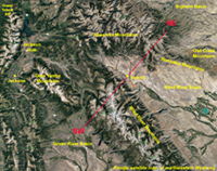 Fig. 3-40. Satellite view of northwestern Wyoming showing location of cross-section line in Fig. 3-42. Fig. 3-40. Satellite view of northwestern Wyoming showing location of cross-section line in Fig. 3-42.
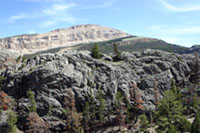
Fig.
3-41. View of Torrey Canyon in the Wind River Mountains near Dubois, Wyoming.
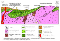
Fig. 3-42. Cross section of the Wind River Mountains and Basin region, Wyoming. |
3.17
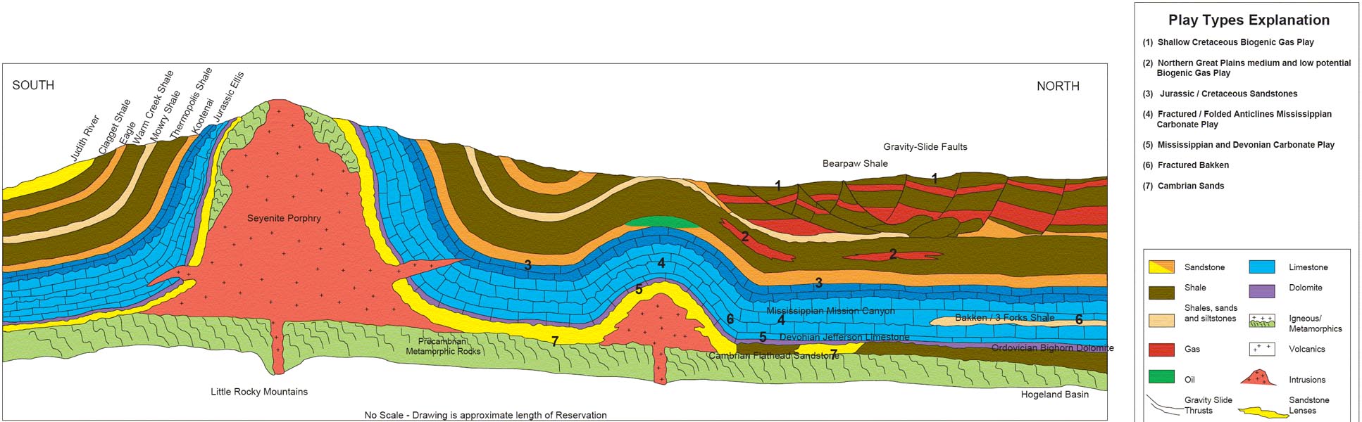
Cross Section of the Little Rocky Mountains Region of Montana
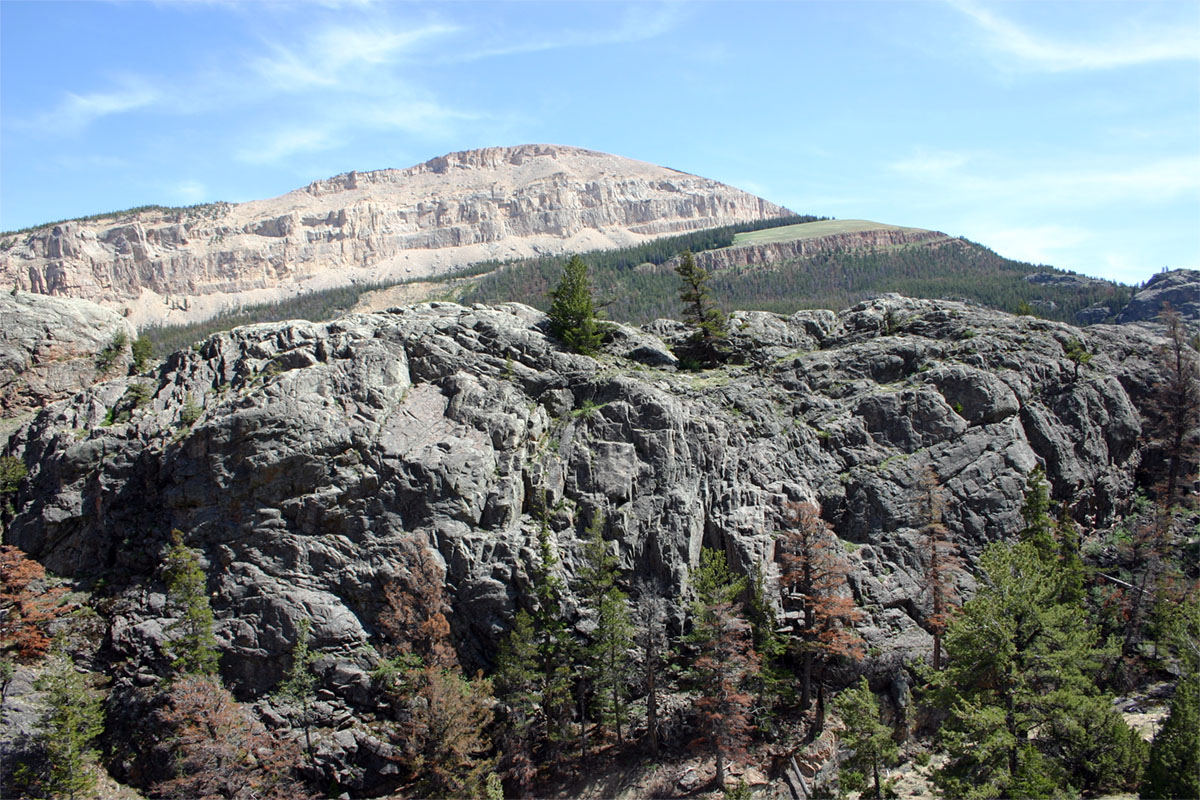
Figure 3-43 illustrates a cross section trending north-to-south across a mountain range in central Montana. The diagram shows two large (red) igneous intrusions that formed when magma pushed up and created two large bubble-like bodies (magma chambers) beneath older layers of sedimentary rocks (blue, orange, and brown). Erosion long after the igneous activity stripped away rocks, exposing steeply dipping layers of layered sedimentary rocks exposed on the flanks of the high peak of the mountain range.
|
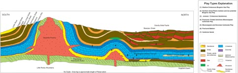 Fig. 3-43. Cross section of Little Rocky Mountains, Montana. Fig. 3-43. Cross section of Little Rocky Mountains, Montana. |
3.18
Cross Section of the Southern San Francisco Bay Region
Figure 3-44 shows a cross section through the Santa Cruz Mountains, Santa Clara Valley, and Diablo Range in the vicinity of San Jose California. The cross section represents a distance of about 30 miles, the vertical is highly exaggerated to highlight the landscape features.
The cross section shows a complex series of faults that separate great blocks of rocks of mixed ages and compositions in the region. In this case, relative dating at least shows that the faults are younger than the rocks they cut through. However, other means would be necessary to explicitly date the age of the rocks and the (younger) faults. |
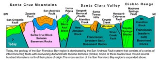
Fig. 3-44. Cross section of the South Bay region, California showing major faults between great blocks of rocks of different age and origin.
|
3.19
Cross Section - Relative Dating Interpretation Exercise |
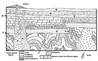
Fig. 3-45. Geologic cross section exercise. |
Use the Laws of Original Horizontality, Superposition, and Cross-Cutting Relationships and unconformities to interpret the order of the formation of features illustrated in this hypothetical cross section (Figure 3-45). Be sure to review Figures 3-19 and 3-21,
Note that a legend on the bottom of the cross section indicates different kinds of rocks illustrated in the cross section.
Letters on the cross section indicate geologic features including sedimentary rock layers, igneous intrusions, faults, and unconformities (lines representing periods of erosion and non-deposition).
Create a list (letters A to P) of the "events" in order as they occurred, from oldest to youngest.
The answers to this exercise are posted at the end of this chapter (below). |
3.20
Absolute Dating Methods
Absolute dating is a general term applied to a range of techniques that provide estimates of the age of objects, materials, or sites in real calendar years either directly or through a process of calibration with material of known age.
There are many methods of absolute dating rocks or other ancient materials. The methods of absolute dating used depends on whether suitable sample are available for testing.
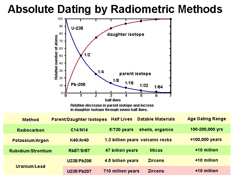
One variety of absolute dating methods involves the study of the decay of radioactive isotopes. The original isotope is the "parent" which through radioactive decay becomes the "daughter" isotope. Commonly referenced studies of absolute dating utilize the radioactive decay of 238U (unstable uranium isotope) into 206PB (stable lead isotope); or 40K (unstable potassium isotope) into 40Ar (stable argon isotope). Note that here are many other absolute dating methods. Perhaps most important is radiocarbon dating which utilizes the decay of 14C (unstable carbon isotope) into 14N (stable nitrogen isotope). Dating of materials that contain naturally-occurring radionuclides (radioactive isotopes) is possible because the rate of decay of the radionuclides are known. The radiation decay "clock" starts the moment a mineral in a rock forms (or for 14C when an organism dies).
Figure 3-46 shows information about several absolute dating methods. Each method uses different parent/daughter isotopes. Each method has a suitable age dating range and materials that can be dated (such as minerals, shells, organic mater, etc.). It is important to note that today there are dozens of other absolute dating methods using a variety of technological innovations. A half-life is when only half of a parent radionuclide remains. The next half-life is when only a quarter of the original parent radionuclide remains, and so on. Age determinations can be determined by comparing the percentage of the radionuclides in a new "fresh" sample with the percentage in the old sample material being tested.
|
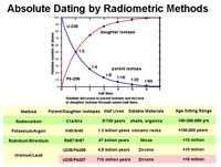 Fig. 3-46. Absolute dating methods. Different isotopes are used to study different materials and geologic time ranges. This diagram illustrates the concept of half lives of decaying radioactive elements commonly used in many absolute dating methods. Fig. 3-46. Absolute dating methods. Different isotopes are used to study different materials and geologic time ranges. This diagram illustrates the concept of half lives of decaying radioactive elements commonly used in many absolute dating methods. |
3.21
Absolute Dating of Moon Rocks
Six Apollo Mission space craft landed to the Moon (1969-1972). The missions returned with about 820 pounds (382 kilograms) of moon rocks. Figure 3-47 shows one of the largest samples, a medium-grained olivine basalt collected by Apollo 15 astronaut, Dave Scott, who collected the sample from the rim of Hadley Rille on August 2, 1971. The collection of the moon rocks was a driving force for finding new absolute dating methods for rocks, like these very-expensive samples. Absolute dating studies of the moon rocks show that most of the sample range in ages between about 3.16 billion years for rocks from the Moon's Mar regions, to as old as 4.4 billion years for older rocks exposed in the more ancient Lunar Highlands regions. The older moon rock samples are older than any rocks yet found on Earth.
Absolute dating studies of the sample shown in Figure 3-47 has resolved that the rock came from an eruption of molten material from the ancient Moon's mantle about 3.3 billion years ago. The current age of the origin of the Moon is 4.51 billion years. |
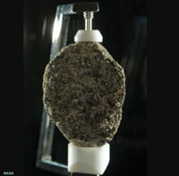 Figure 3-47. A sample of a moon rock collected on the Apollo 15 Mission of 1971. Figure 3-47. A sample of a moon rock collected on the Apollo 15 Mission of 1971. |
3.22
Radiocarbon Dating
14C (isotope carbon -14) is a unstable radioactive isotope of the element carbon (a radionuclide). Radiocarbon dating involves using ratios of the isotopes of radioactive isotope14C to stable isotopes 12C and 13C derived from buried or isolated organic or carbonate materials. Figure 3-48 illustrates the science behind radiocarbon dating. The half life of 14C [unstable isotope carbon-14] is about 5,730 years. Radiocarbon dating has extensively used in archaeological investigation and the study of climate change over the last several hundred thousand years, and precision methods now available make radiocarbon dating highly reliable. Radiocarbon dating is highly effective for extracting ages of organic materials (bone, tissues, wood, etc.) that have been isolated from the atmospheric interactions by burial. Radiocarbon dating is widely used and has proven particularly effective for dating materials from ancient archaeological sites to date human activities going back for many thousands of years.
|
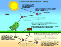
Fig. 3-48. The science behind the radiocarbon absolute dating method. |
3.23
3.24
Maps are useful for any profession, but they are particularly important to the natural sciences, especially geology.
Geologic maps and topographic maps are perhaps the most important tools for evaluating landscapes for a host of issues involving land use, natural resources, and interpreting the geology both above and below the surface. Maps have been used well back into prehistoric times. However, the evolution of maps in the modern digital world has significantly changed map making—enhancing their use in nearly all aspects of modern science, technology, and culture. Modern maps are created with geographic information systems (GIS for short)—computer-based map-generating programs can combine geographic (spatial) information with many kinds of databases (medical, commercial, civic infrastructure, biological, geological, satellite data, etc.). Whether printed on paper or in a digital format, geologic maps are essential to understanding local and regional geology, including natural resources (minerals, water, soils) and natural hazards (earthquake faults, volcanic hazards, flooding and landslide hazards). |
Click on images for a larger view throughout this website. |
 |
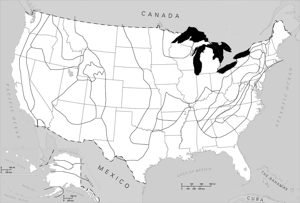
| Fig. 3.49. A blank line map of US is always useful! |
3.25
What is a map?
A map is a diagrammatic representation of the land surface (or part of it), showing the geographical distributions, positions, and names of natural or artificial features such as roads, towns, relief, rainfall, etc. Maps are a scaled, 2 dimensional representation of the surface of an area or region. Some maps attempt to portray 3-dimensional landscape features, such as mountains or canyons. Maps may represent the surface of the land or regions in and around lakes and oceans, the seafloor, or features known or inferred to occur underground. Mapping is also used in astronomy (planet and moons, regions of space, etc.). There are many kinds of maps. Anything that has a visual distribution on the ground can be mapped.
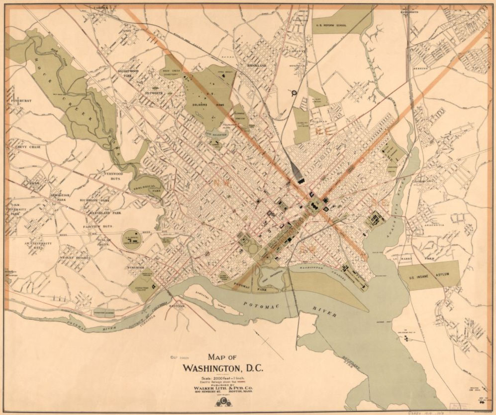
Prior to the modern digital world, maps were static sources of information, providing a glimpse of what existed in an area at the time that a map was compiled (example, a century old map of Washington DC is no longer accurate, but has historic value, Figure 3-50). In our modern world, maps can be updated with real-time information, but like all information, the data provided may have limited accuracy or scope, and may have bias to exaggerate or withhold selected information. |
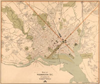
Fig. 3-50. Map of Washington, D.C.:
Boston: Walker Lith. & Pub. Co., [1910?]. Library of Congress Photoarchive. |
3.26
Thematic Maps
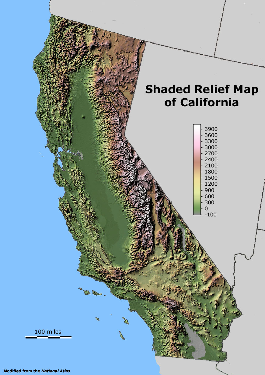
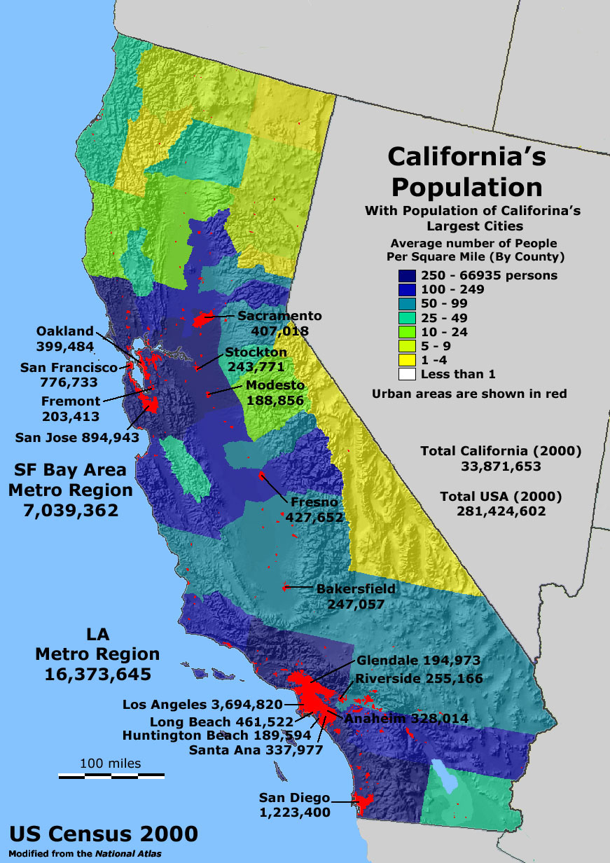
A thematic map is is a map with a special theme applied to a geographic area. Themes can include physical geography, social, cultural, political, economics, land use, natural resources, hazards, or practically any data that can be presented geographic form, and on any scale, such as town, city, state, country, continent, or the world. Below are 12 examples of different thematic maps for the state of California (Figures 3-51 to 3-64). |
Selected Thematic Maps of California |
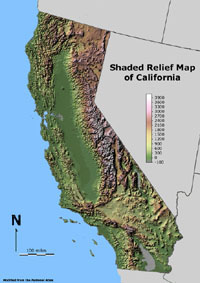
Fig. 3-51. Shaded relief map of California (elevation is expressed in color variations) |
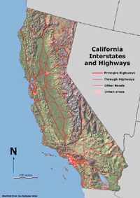
Fig. 3-52. California interstates and highways with cities on shaded relief map |

Fig. 3-53. California population density by county and largest largest cities |

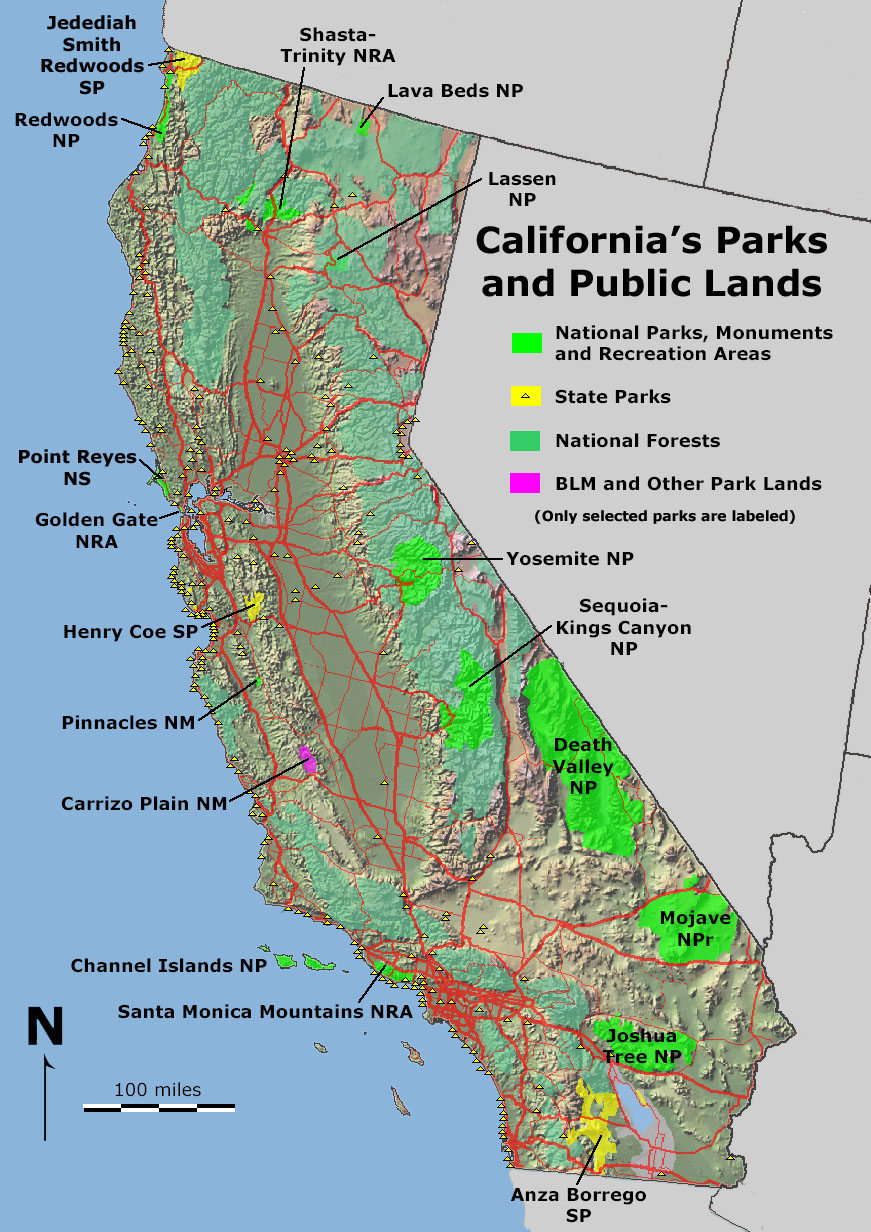
Fig. 3-56. California's parks and public lands (showing state and national parks) |
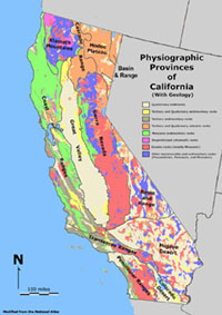
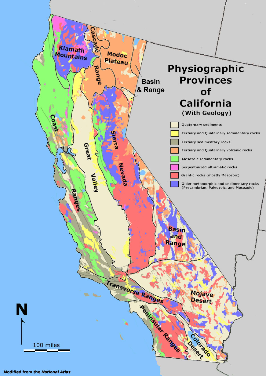
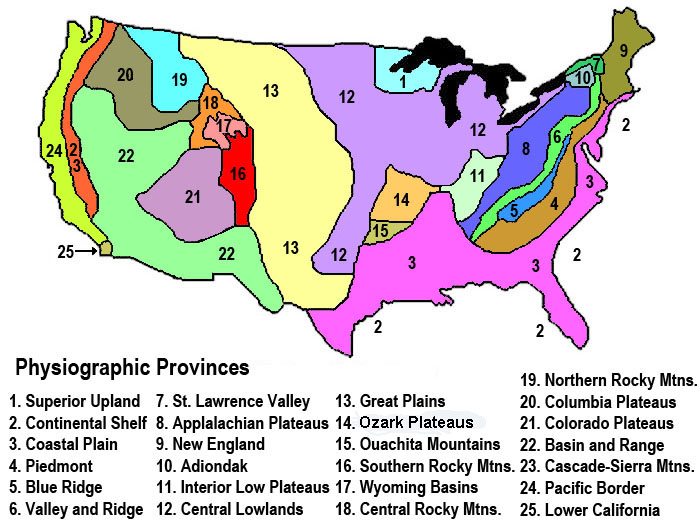
Fig. 3-57. Physiographic Provinces of California (with geology)
|
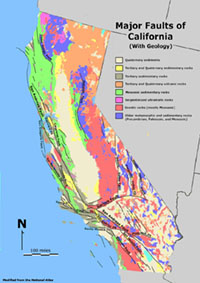
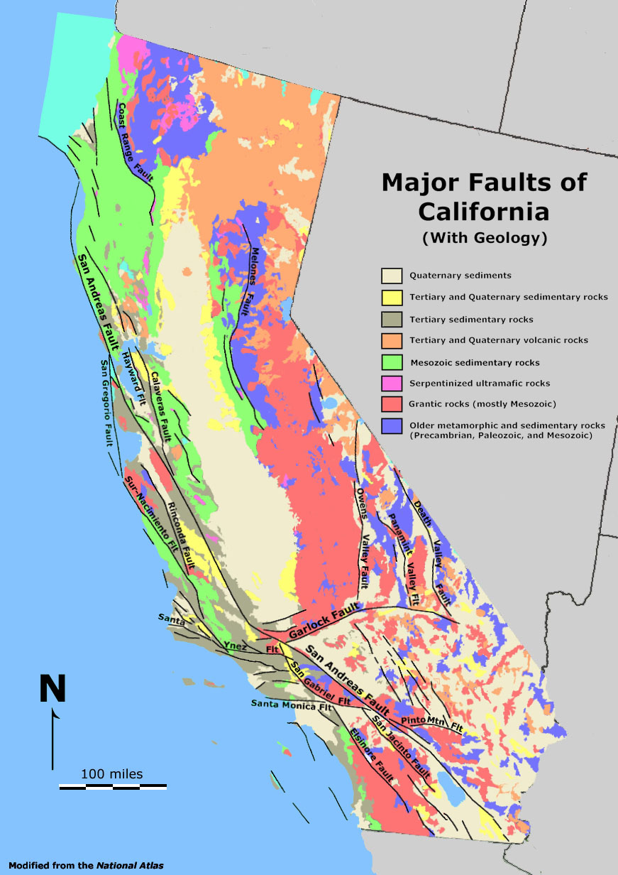
Fig. 3-58. Major faults of California (with geology)
|
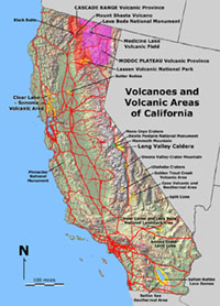
Fig. 3-59. Volcanoes and volcanic areas of California (with cities, roads, and relief) |
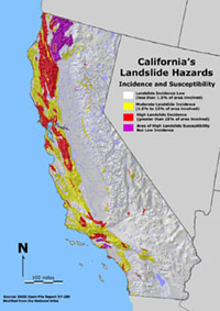
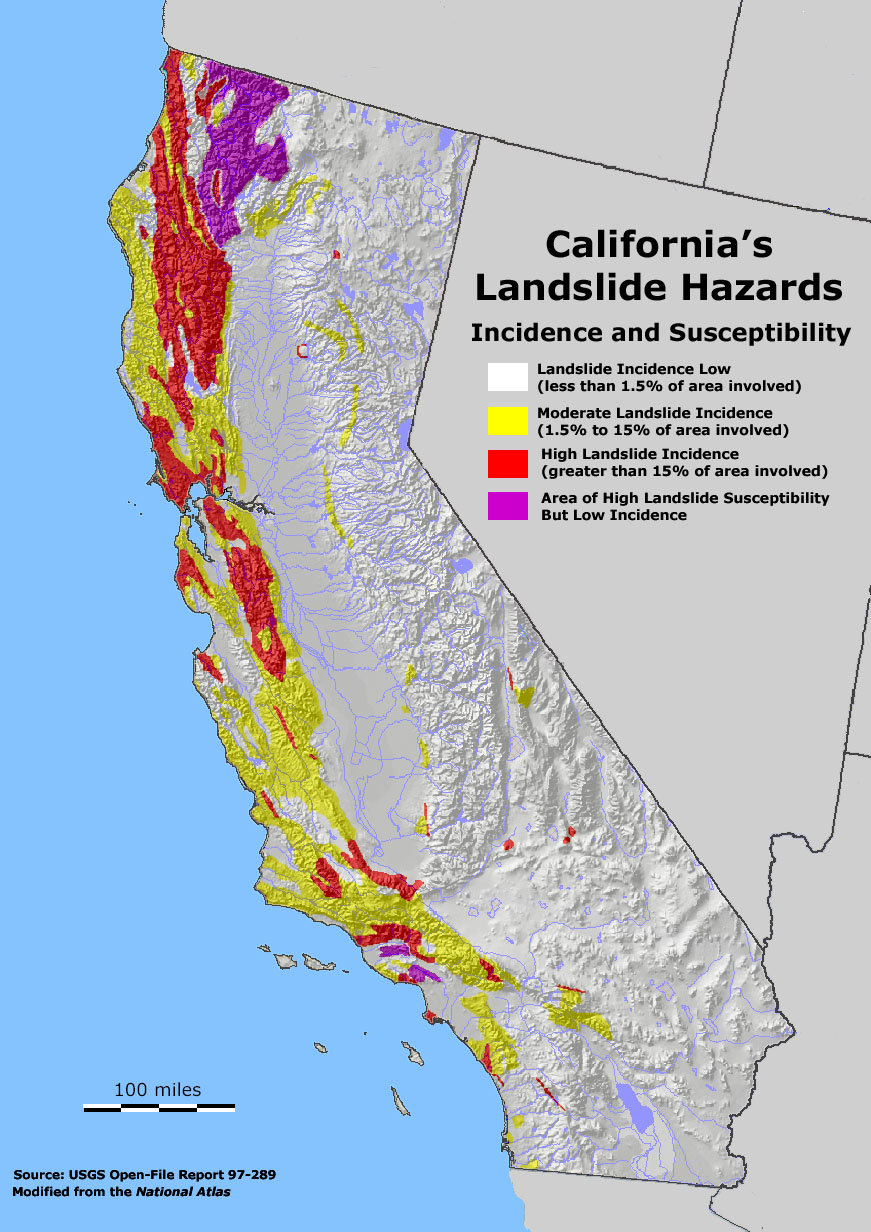
Fig. 3-60. California's landslide hazards map (susceptibility). |

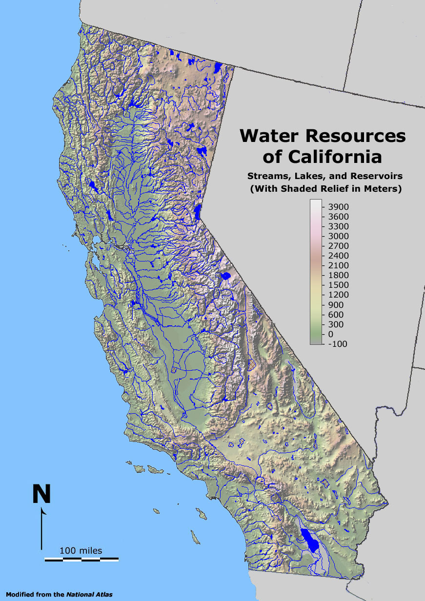
Fig. 3-61. Water resources of California (with water and shaded relief)
|
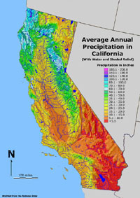
Fig. 3-62. Average annual precipitation in California (with water and shaded relief) |
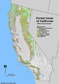
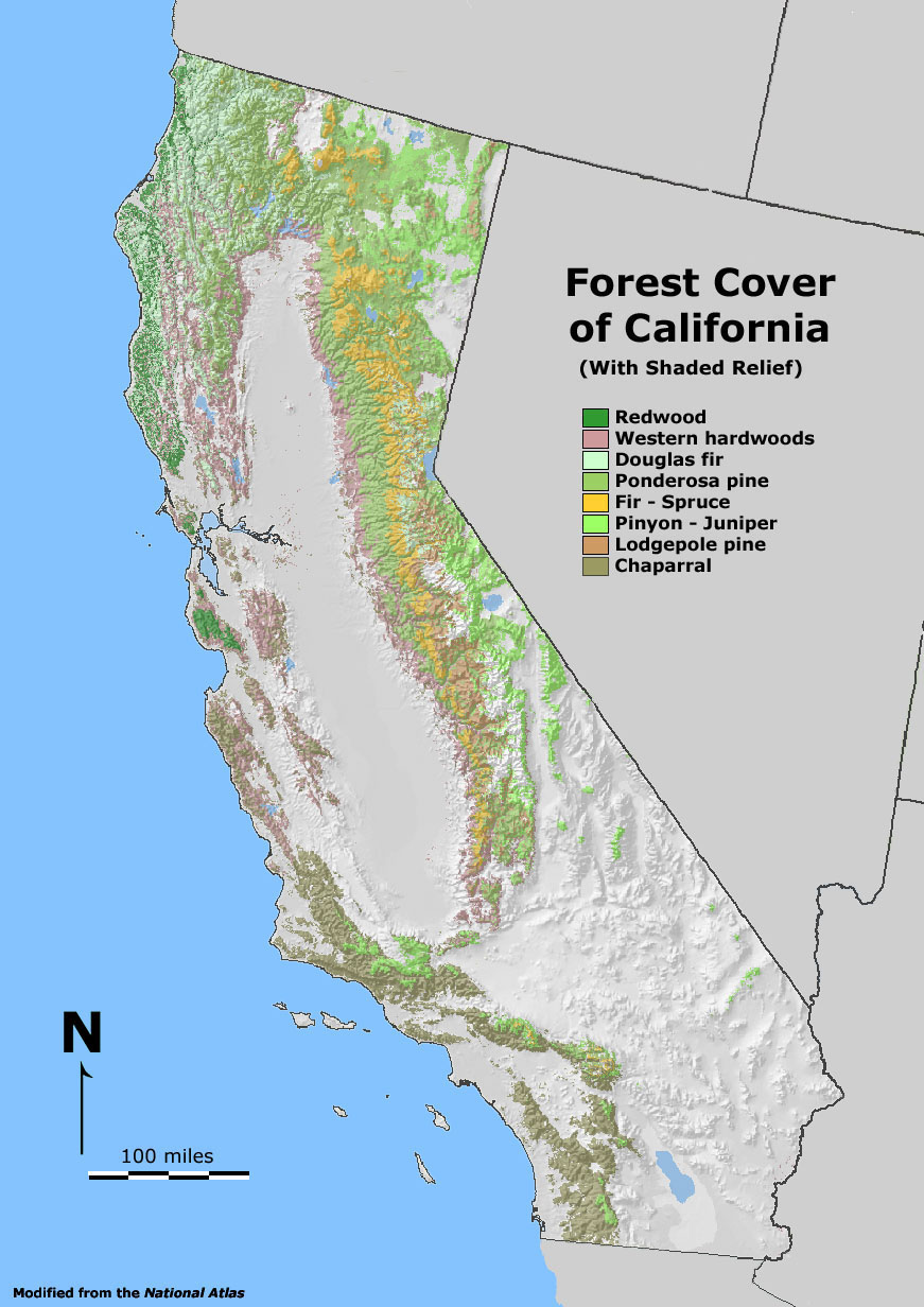
Fig. 3-63. Forest cover of California on shaded-relief map
|
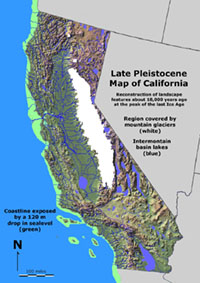
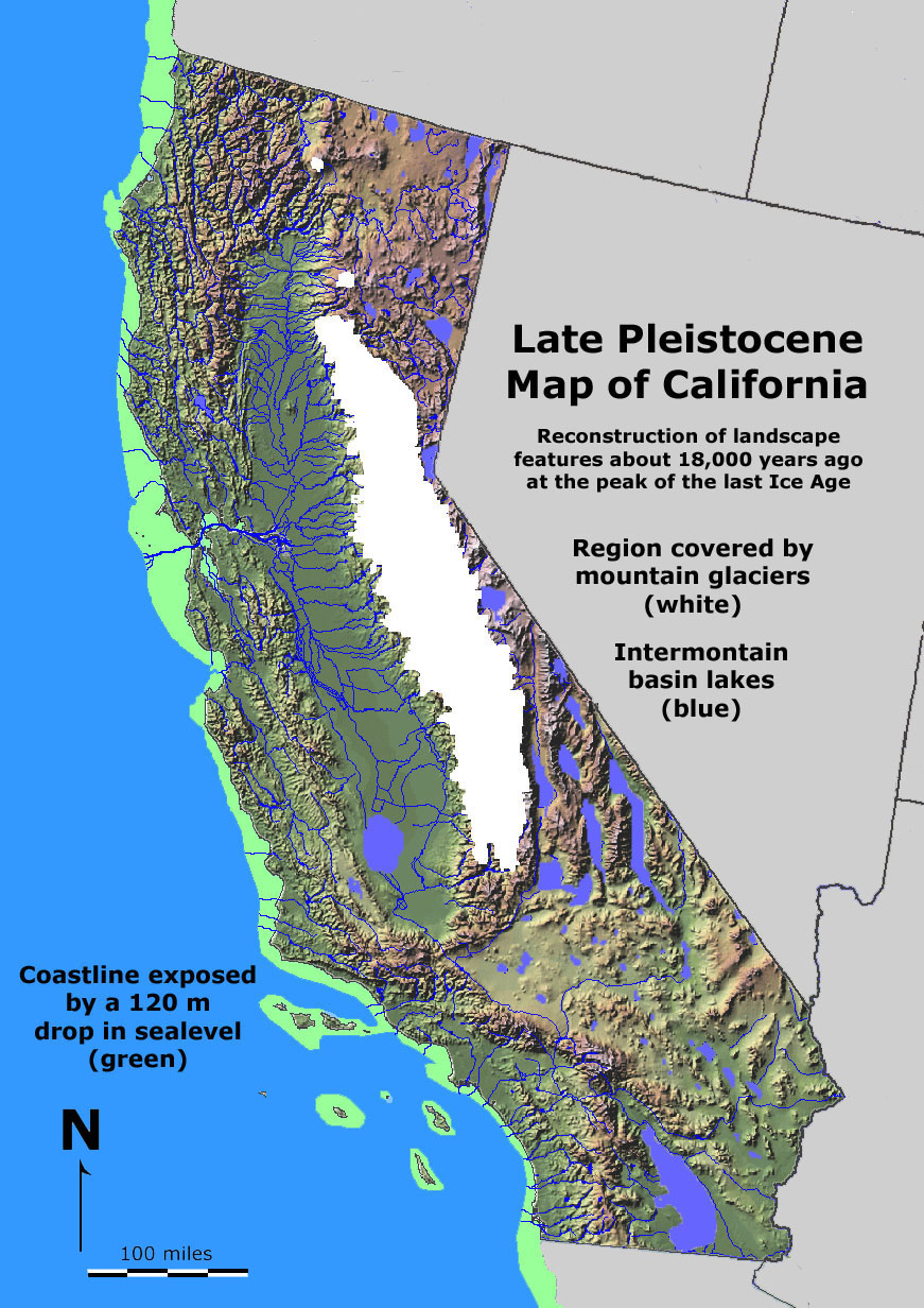
Fig. 3-64. Late Pleistocene map of California (peak of last ice age, 18,000 years ago) |
|
3.27
All Maps Should Include Descriptive Information
Before studying or preparing a map, it is important to examine information about the map. Below is a list of information typically associated with maps. Some of these topics are examine in more detail is sections that follow.
| title |
A title should include concise information related to geographic information and theme (focus) of the map's content. |
| scale |
Map scale refers to the relationship (or ratio) between distance on a map and the corresponding distance on the ground. Scale should be relative to both miles and kilometers, example: 1:24,000. A map should have a visual scale bar to show relative distance on a map. |
| orientation |
Maps should include a north arrow and, if possible, corner coordinates information (longitude & latitude) |
| legend |
Maps need an explanation of symbols used on map, including colors, lines, icons, and special symbols. |
reference
features |
Maps should included selected reference locations or features for orientation (such as cities, towns, highways, state boundaries, coastlines, mountain peaks, rivers, etc.) |
| source information |
A maps authors, compilers, editors, and publishers, associated publications (text or guidebook), URL, and any other information to provide complete information so it can be accurately cited in reference list or bibliography. |
| base map information |
What was the source of geographic information used as the base (background) of a map, such as a USGS topographic map or s NASA satellite image? What is the map projection? |
| date published |
What year was the map released (or revised). Is the data it shows from new or old data sources? |
| written text |
Is there a publication (pamphlet or guide book) associated with this map? |
|
3.28
Topography and Bathymetry
Many maps include information about the elevation differences on maps such feature as mountains, canyons, hills, shorelines, etc.
● Topography refers to the arrangement of the natural and artificial physical features of an area.
● Bathymetry refers to the measurement or mapping of water depth (sea bed) beneath oceans, lakes, or other bodies of water.
Relief is the variation in elevation on the surface of the Earth (topography). Areas of "high relief" have much elevation changes over distance, such as mountainous areas and canyons. "Low relief" occurs where elevation changes are minimal, such as on coastal plains (Figure 3-65).
On maps, both topography and bathymetry
are described as elevations relative the mean sea level in a region. Sea level is reported as 0 (zero) feet, meters, or fathoms (a fathom is 6 feet of water depth).
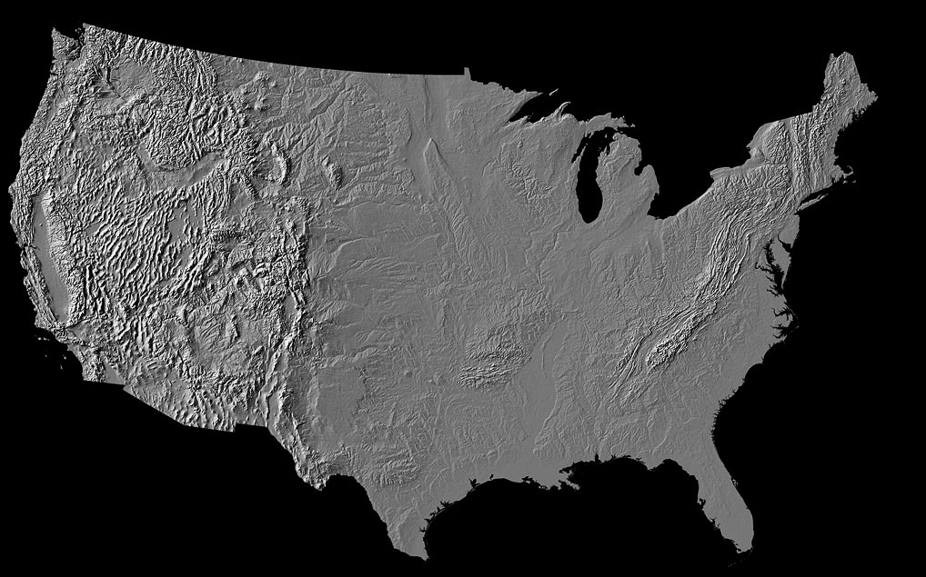
Both topography and bathymetry can graphically illustrated with shaded relief or with contour lines. A shaded-relief map uses gray-scale shading giving the appearance of relief similar to sun shading (the way sunlights highlights a natural landscape—something that our brain automatically understands and processes!). A shaded-relief map can be used to illustrate both topography and bathymetry (Figure 3-66).
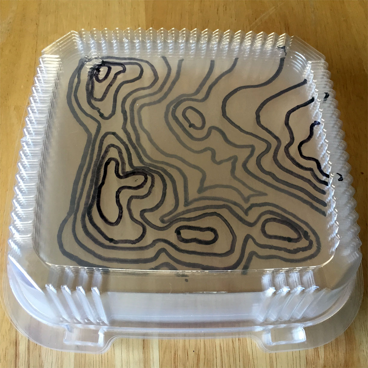
Contour lines are another way to illustrate relief. Contour lines follow points of equal elevation and are spaced at uniform distances apart on a map. Examples of contour intervals might be 10 or 40 feet (or meters), depending on how much relief is in a map area. For example, contour lines can be illustrated by lines drawn on a stack of clear plastic box lids (Figure 3-67). Each lid represents a separate contour—a line of equal elevation.
A topographic map is a graphical representation of a landscape showing selected natural and artificial landscape features including topographic relief. A topographic map shows many features including relief (contours) and man-made features of a portion of a land surface distinguished by portrayal of position, relation, size, shape, and elevation of the features (see example in Figure 3-68). The US Geological Survey produced topographic maps on many scales from the late 19th Century to the end of the 20th Century. Now, nearly all information is now in digital data provided by satellite information and other sources (discussed below).
A map of the bathymetry of the ocean floor or large lake is called a chart. |
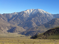
Fig. 3-65. A region of high relief is illustrated by this mountainous mountain face on San Jacinto Peak near Palm Springs, California. The alluvial fan in the valley below the peak is a region of low relief.
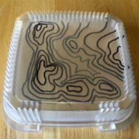 Fig. 3-67. Contours lines are lines that show levels of equal elevation. This figure illustrates contour lines drawn on on a series of a stack of six clear plastic box lids. Each lid has a separate contour line. This visually recreates three dimensional relief model as represented by contour lines on a topographic map. See examples of contour maps used to create similar examples of stacked box lids. Fig. 3-67. Contours lines are lines that show levels of equal elevation. This figure illustrates contour lines drawn on on a series of a stack of six clear plastic box lids. Each lid has a separate contour line. This visually recreates three dimensional relief model as represented by contour lines on a topographic map. See examples of contour maps used to create similar examples of stacked box lids. |
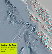
Fig. 3-66. A shaded relief map of the central coast of California including Monterey Bay and San Francisco, CA. Both topography (on land) and bathymetry (undersea) are shown.
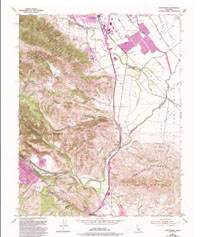
Fig. 3-68. Example of a USGS topographic map: Chittenden, CA 7.5 minute quadrangle.
This map is an example of a map that the US Geological Survey produce for the United State for over 100 years before our modern map technology. |
3.29
What are Latitude and Longitude?
Locations on the Earth's surface are defined using latitude and longitude coordinate system.
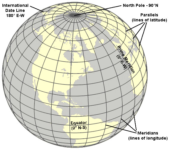
Latitude is a measure of the angular distance of a place north or south of the Earth's equator, usually expressed in degrees and minutes. Lines of latitude are called parallels. Latitude lines are parallel to the Equator. Each degree of latitude is approximately 69 miles (111 kilometers) apart (Figure 3-69).
| There is 90 degrees of latitude between the Equator and the North Pole. There are 60 minutes with each degree. Each minute equals 1 nautical mile. One nautical mile is 6,076 feet. When examining the globe, simple math shows that 90 degrees (the degrees of latitude difference between poles and Equator) times 60 nautical miles (per degree) is a distance of 5,400 nautical miles. For comparison, one nautical mile equals 1852 meters. One mile is 5,280 feet; a nautical mile is equal to 1.15078 miles. |
Longitude is a measure of the angular distance of a place east or west of the Prime Meridian, and is also expressed in degrees and minutes. In order to make an accurate map of the stars for use in ship navigation, an important decision was made in 1884 to establish a longitude grid for Earth. A location indicating the precise location of 0° East-West longitude was designated in the cross hairs of a telescope in the Royal Observatory in Greenwich, England. (The Royal Observatory is located on the grounds of the National Maritime Museum in London). This Prime Meridian marks the north-south reference location used in all global mapping (including GPS location systems).
A meridian is a circle of constant longitude passing through a given place on the Earth's surface and the terrestrial poles. Longitude lines (lines of equal spacing measured in degrees) are widely spaced at the equator, but converge at single points at both the North Pole and South Pole where all the meridians intersect (Figure 3-69).
The Prime Meridian is designated 0° (zero degrees). Meridian lines east of the Prime Meridian are designated positive values (0° to 180° east); whereas meridian lines west of the Prime Meridian are designated negative values (-0° to -180°). At 180° east or west is the International Date Line. A degree of longitude is widest at the equator at 69.172 miles (111.321) and gradually shrinks to zero at the poles. At 40° north or south the distance between a degree of longitude is 53 miles (85 km).
Defining locations with a latitude-longitude coordinate system—any location on the planet surface can be defined by a number in degrees and minutes north or south of the Equator and east or west of the Prime Meridian. For more detail, minutes are divided into seconds for more precise location with the longitude-latitude designation (compared with hours, minutes, and seconds on a clock!) |
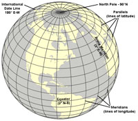
Fig. 3-69. Latitude and longitude projected on a globe.
Parallels (lines of latitude) are circles parallel to the Equator. Each circle north or south of the Equator are increasingly smaller (shorter).
Lines of latitude start at 0º at the Equator, and increase to 90º north at the North Pole, and 90º south at the South Pole.
Meridians (lines of longitude) converge on the poles.
Lines of longitude start at 0º (degrees) at the Prime Meridian and increase to 180º east or 180º west to the International Date Line. At 180º E or W, the International Date Line is located in the middle of the Pacific Ocean.
|
3.30
Plotting Latitude and Longitude On a Map
Latitude and longitude are reported in two ways: as standard coordinates or decimal degrees.
Standard coordinates are the older method of using degrees, minutes, and seconds [DMS]). This method of reporting location was important before modern shipping navigation systems became available.
Decimal degrees report latitude and longitude degree values using positive or negative numbers with decimal fractions (not minutes and seconds). Positive latitudes are north of the Equator, negative latitudes are south of the Equator. Likewise, positive longitudes are east of the Prime Meridian, and negative longitudes are west of the Prime Meridian.
The modern reporting using GPS (Global Positioning System) is to combine standard coordinates and decimal degrees, abandoning the confusing positive or negative symbols and using north, south, east, and west direction designations.
|
Example: Location of the Statue of Liberty in New York Harbor
The standard coordinates of the Stature of Liberty are:
Latitude: 40°68′92" N
Longitude: 74°04′ 45" W
Described in decimal degrees the coordinates of the Statue of Liberty are:
Latitude: 40.689758°
Longitude:-74.045138°
Coordinated decimal degrees used by most modern GPS devices (on mobile phones) for of the Statue of Liberty are:
Latitude: 40.689758° N
Longitude: 74.045138° W |

Fig. 3-73. The Statue of Liberty is a landmark located in New York Harbor between New York and New Jersey. |
3.31
Map Projections
Trying to make a flat map of a round planet is like trying to fit a square peg in a round hole. Noting fits perfectly.
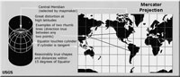
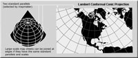
The Earth is round (a sphere like a globe) but paper maps are flat. As a result, maps that show large regions are distorted. Map projections are attempts to portray a portion of the earth on a flat surface. The flattening of a map always causes some distortions of distance, direction, scale, and area. Large scale maps (such as a map of a continent or a world show much distortion. In contrast, maps on small scales (such as a map of a town or neighborhood) have relatively little distortion. The Mercator Projection is perhaps the most widely used in flat-map publications (Figure 3-71).
|
 |
 |
|
| Fig. 3-70. A global view of a planet is the only way to have perfect map projection! |
Fig. 3-71. Map of world showing with Mercator Projection - notice distortion in high latitudes because longitude lines are not converging as on a globe. |
Fig. 3-72.
Map of North America with Lambert Conic Projection - on this scale distortion of America is minimal, but look at South America. |
|
3.32
The Mercator map in Figure 3-74 is an example of a general Mercator map for pin-pointing latitude and longitude.
Below are examples of the GPS location of points representing major cities as reported on a Google search for coordinates. Note that these reported coordinates are subjectively reported -- because cities are large areas, covering hundreds of square miles. It is unclear what these points may represent in each of the cities listed below. Compare these coordinates with the map in Figure 3-74. Note that these locations listed below are the coordinated GPS decimal degrees reporting method.
New York City, USA: 40.7128° N, 74.0060° W
Rome, Italy: 41.9028° N, 12.4964° E
Buenos Aires, Argentina: 34.6037° S, 58.3816° W
Melbourne, Australia: 37.8136° S, 144.9631° E |
Find a latitude and longitude of any named location or landscape feature on the GeoNames website. |
|
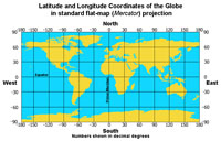
Fig. 3-74. Map of the world showing latitude and longitude in a Mercator (flat) projection with numbers illustrated in decimal degrees. |
3.33
The Global Positioning System
A Global Position System (GPS) is a system of Earth-orbiting satellites synced with computers and universal atomic time clocks that send information to receivers, such as a cell phone, car, or hand-held GPS. GPS devices are capable of measuring precise latitude, longitude, and elevation of a receiver anywhere on Earth. Locations are calculated by comparing the time delay for signals to reach a ground-based receiver from different satellites. Real-time calculations can provide precise determinations of the location of the receiver.
Most modern mobile telephones have GPS connectivity.
The GPS system was developed, funded, and is controlled by the U.S. Department of Defense. The GPS system was made public in 1995 and has undergone extensive development with at least two-dozen satellites, and is currently used for thousands of civilian applications worldwide. Real-time GPS is used for navigation to determine exact location, velocity, and time anywhere around the world. GPS provides reliable location and time information in all weather conditions and at all times, anywhere on or near the Earth when and where there is an unobstructed line of sight to four or more GPS satellites. |
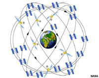
Fig. 3-75. The Global Positioning System (GPS) of satellites orbiting Earth. |
3.34
Earth's Rotation Influences It Shape
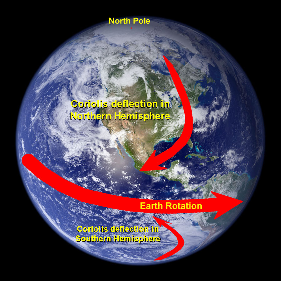
From space, Earth may look like a perfect sphere; however, detailed measurements show that the planet is not a perfect sphere. Earth's rotation impacts the shape of the Earth. The circumference of Earth at the Equator is 24,902 miles (40,075 km, or 21,639 nautical miles). In contrast, the meridional circumference ( longitude lines following the great circles that converge at the poles) is only 24,860 miles around (or 40,008 km or 21,603 nautical miles). This is because the Earth is spinning—this rotation causes the Earth to expand at the equator, and flattens at the poles. Because of the spinning, Earth is actually an oblate spheroid, not a perfect sphere. At the poles, there is rotation, but no motion. In contrast, at the Equator, the Earth surface is moving about 1,000 miles per hour (460 meters per second) toward the east. This difference in physical motion between the poles and equator is responsible for dynamic rotation forces, called the Coriolis effect. The Coriolis effect is responsible for the observable rotation in currents driving oceanic and atmospheric systems, including atmospheric rotation in hurricanes (discussed with relevant topics in following chapters, Figure 3-76). |
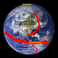
Fig. 3-76. Earth's spin influences the shape of the planet and causes the Coriolis effect. |
3.35
Important Historical Mapping In the United States
As the United States expanded westward across North America into new territories, the Federal government developed the Public Land Survey System (PLSS) to chart out the country to subdivide the landscape into rectangular boundaries to establish property boundaries, access routes, and provide a system for naming and locating precise locations on the ground.
While the PLSS worked for subdividing the land, the problem of trying to map and subdivide the land into squares on a curved land surface presented many problems, especially for mapping the nation as a whole. A new method of mapping used by the US Geological Survey involved subdividing regions to be mapped into quadrangles—using latitude and longitude designations for map boundaries (discussed below). |
3.36
The Public Land Survey System
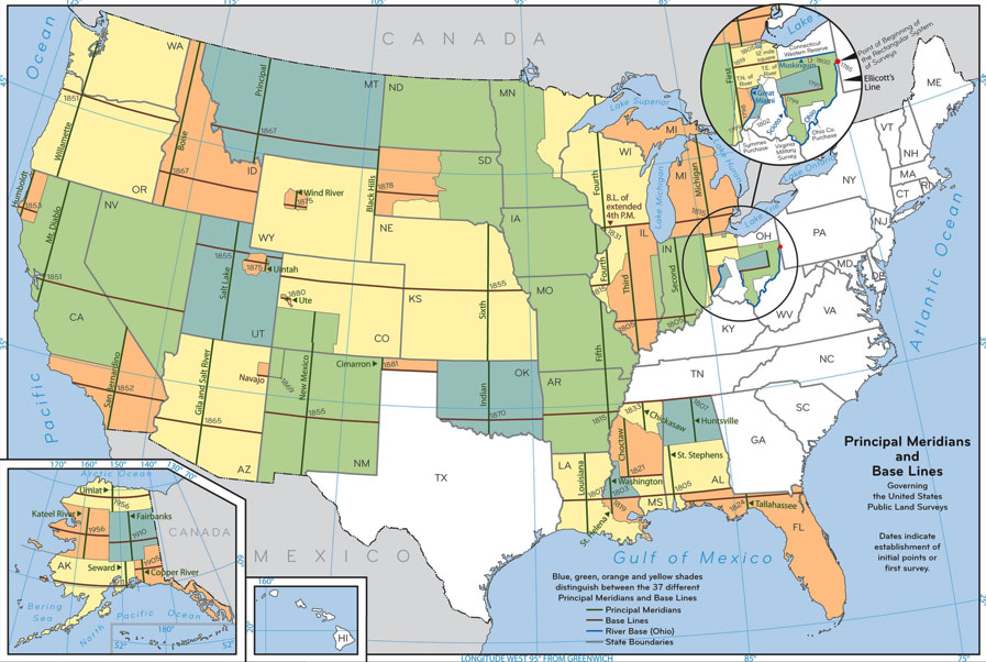
Historically, as the United States expanded its territories in the 18th to early 20th centuries, land was surveyed (mapped) and subdivided using the Public Land Survey System (Figure 3-77). The first use of the PLSS began in Ohio in 1785. The PLSS is still used for all lands in the public domain, and is currently regulated by the Bureau of Land Management (a branch of the U.S Department of Interior).
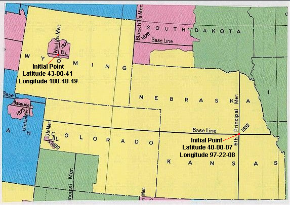
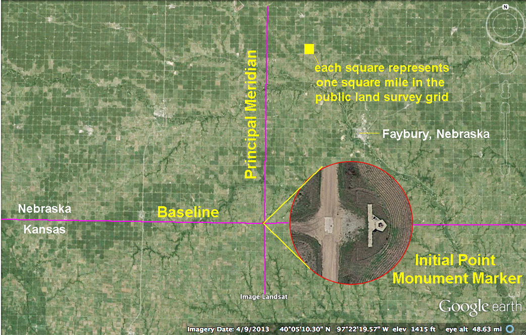
This method of surveying involved measuring a grid of lines east-to-west and north-to-south starting with a designated initial point (such as a mountain peak like Mt. Diablo in central California). From an established initial point, a north-to-south was mapped (called the principal meridian). From the initial point, a baseline was mapped east-to-west following a line of latitude. See examples of the initial point, principal meridian, and baseline for the Nebraska Territory Survey in Figures 3-78 and 3-79.
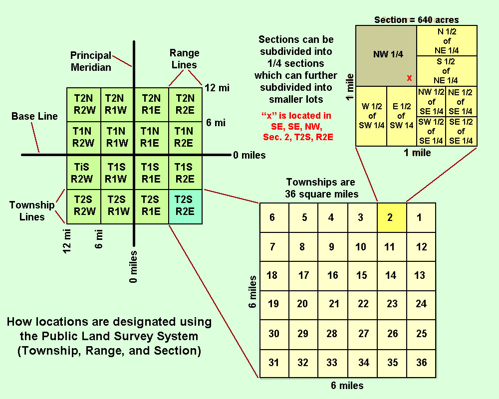
North-south lines are called township lines and east-west lines are called range lines (Figure 3-80). These lines of a grid are parallel mapped at intervals of at 1 mile apart. Flying over the country today it is easy to see the historical significance of the township and range lines because they are the locations of roads and property boundaries throughout the landscape we see today. The geographic term, township, is often square region of land that encompasses 36 square miles as defined by township and range lines (Figure 3-80). One square mile of land within a township is called a section. There are 36 section in one township. Each section is number in a consistent pattern, and sections may subdivided into quarters (labeled NE, SE, SW, NW) and these quarters may be subdivided into quarters, and so on (see Figure 3-80).
On a limited regional scale, township and range lines work fairly well, but with increasing distances the rectangular pattern begins to fail due to distortion caused by the curvature of the Earth surface. To solve the distortion problem, new grids with township and range lines were set up throughout the country over time. The Public Land Survey System is used for describing locations where the land grid has been establish. Throughout much of the United States, particularly in western states, roads (commonly dirt tracks) follow section lines east and west, and north and south. These lines are considered public access routes in most states, and are a means of finding and locating specific pieces of property or locations on public lands. |

Fig. 3-77. Principal Meridians and Base Lines of region that used the Public Land Survey System (map provided from US BLM). |

Fig. 3-78. Detail view of a public land survey of Nebraska Territory showing the initial point, principal meridian, and baseline. |
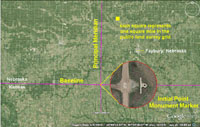
Fig. 3-79. Google satellite image views of the initial point for the Public Land Survey of Nebraska Territory started in 1855. |
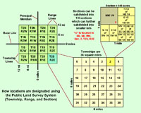
Fig. 3-80. Locations in areas mapped with the Public Land Survey System are designated by township, range, and section. |
3.37
USGS Topographic Maps
The US Geological Survey was established in 1879, and then the US Congress approved topographic mapping of the United States in 1882. For well over 130 years, the USGS conducted topographic mapping across the United States and its territories. This colossal endeavor required map standards (designations of common symbols, scale, contours, etc.) that had to be consistently used for mapping by thousands of mappers over time. Initially, all mapping was done on a scale of 1:48,000 for maps that covered 15 minute quadrangles—maps covering 15 minutes (or 1/4 degree) of latitude and longitude on each side. Later it changed to the 7.5 minute quadrangle standard (with 1:24,000 scale) so as to provide more detail of coverage. In addition, the USGS also provided maps on greater scales (30 x 60 minute maps with 1:100,000 scale, and 1 x 2 degree maps with 1:250,000 scale).
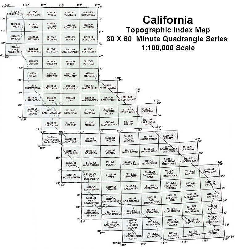
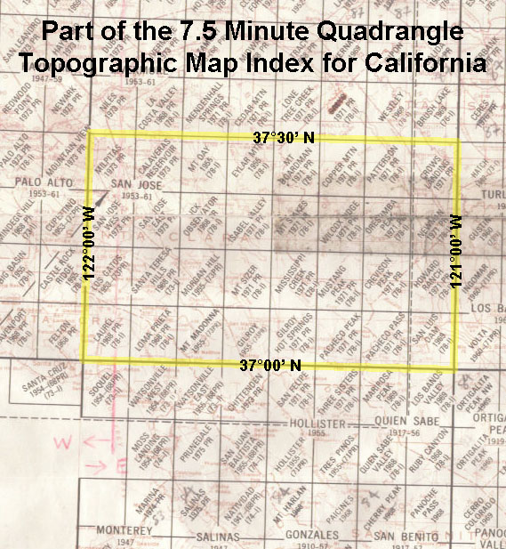
Figure 3-81 is a standard map index for 30 x 60 minute quadrangles for the state of California. Figure 3-82 is a portion of the USGS Topographic Map Index showing the names of 7.5 minute quadrangles. Note that the block highlighted in yellow represents 32 named 7.5 minute subdivisions of one of the quads shown in the 30 x 60 minute map index. [Note that quad is a common abbreviation for quadrangle.] |
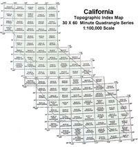
Fig. 3-81. California Map Index for USGS 30 x 60 minute quadrangle designations. (Equals 0.5º latitude and 1.0º longitude on each side of quadrangle map.) |
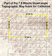
Fig. 3-82. Portion of the California USGS Topographic Map Index showing map 7.5 minute quadrangle designations. |
3.38
Before modern digital mapping, standard USGS topographic maps were 7.5 minute quadrangles with scale of 1:24,000.
The standard USGS 7.5 minute quadrangle map is slightly skewed rectangular-shape representing an area approximately 17 miles (27 km) north to south and within the lower 48 states range from 11 to 15 miles (17 to 24 km) east to west.
There are dozens of different kind of symbols used on topographic maps. See a complete list of US Geological Survey Topographic Map Symbols is at: http://pubs.usgs.gov/gip/
TopographicMapSymbols/topomapsymbols.pdf |
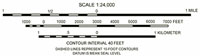
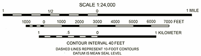
Fig. 3-83. Scale bar on a typical 1:24,000 topographic map (standard USGS 7.5 minute quadrangle maps).
|
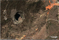
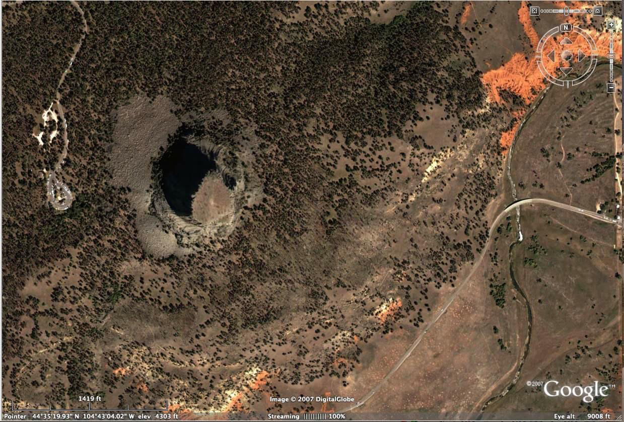
Fig. 3-84. Google satellite view of Devils Tower, Wyoming. Compare this image with a 7.5 minute quadrangle coverage of the same are in Figure 3-84. |
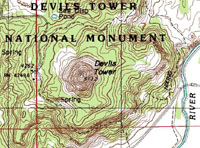
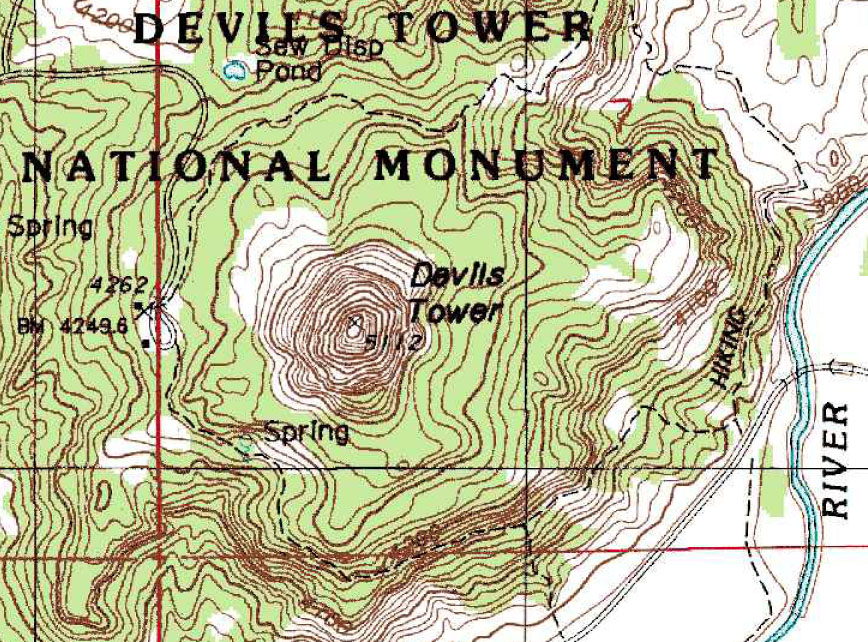
Fig. 3-85. Part of Devils Tower 7.5 Minute Quadrangle Map, Wyoming showing contour lines, green for wooded areas, elevation markers, etc.
|
| On a standard USGS 7.5 minute quadrangle map, one inch on the map is equal to 2,000 feet on the land surface |
3.39
Examples of Topographic Maps
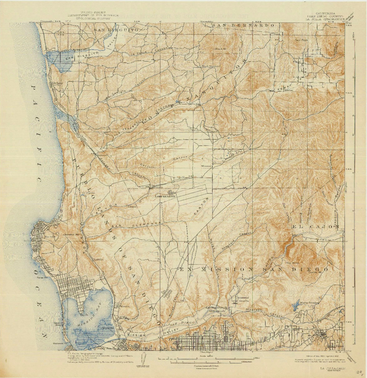
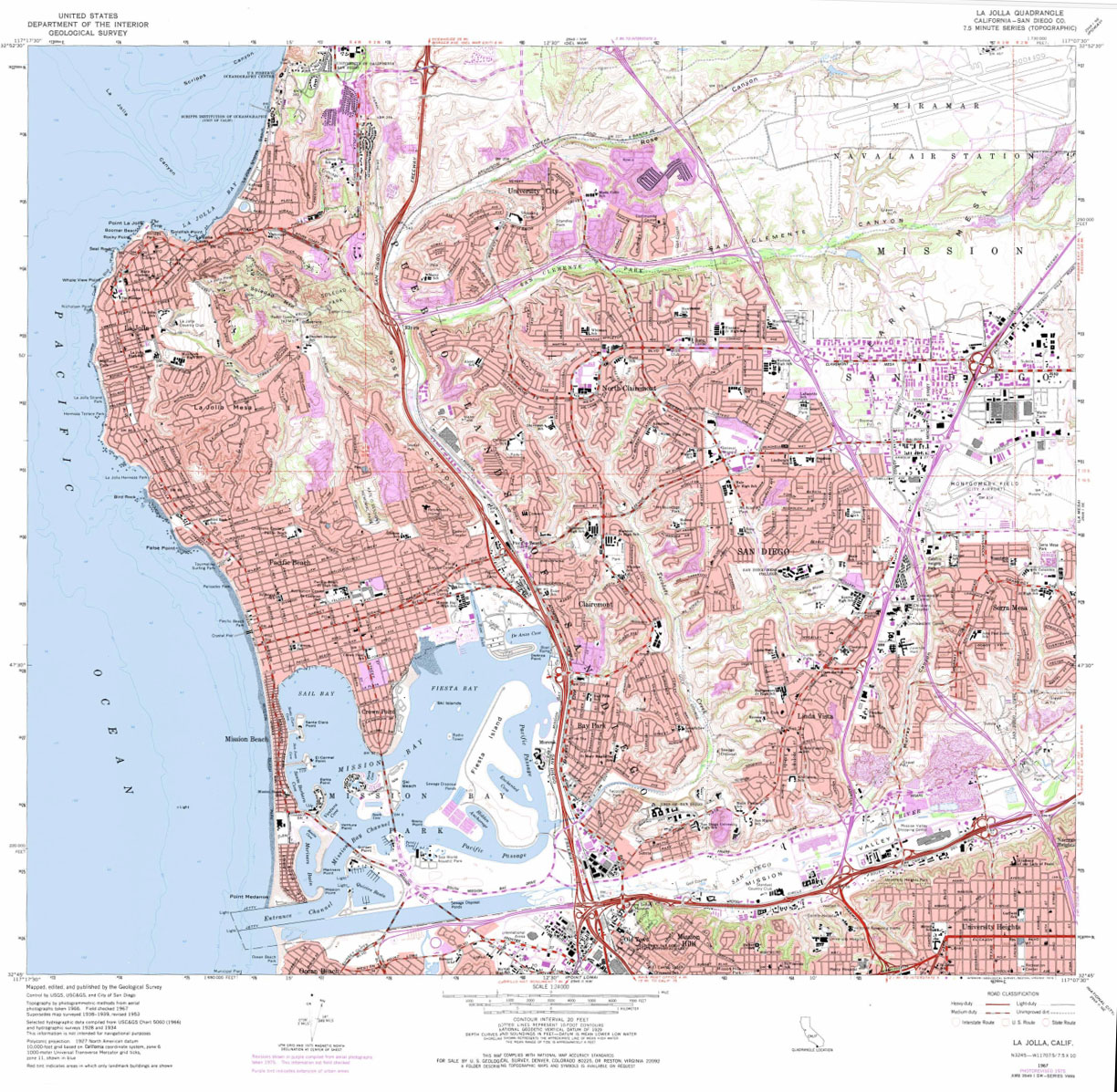
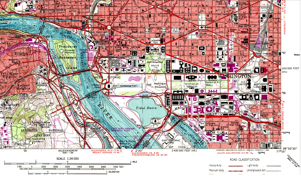
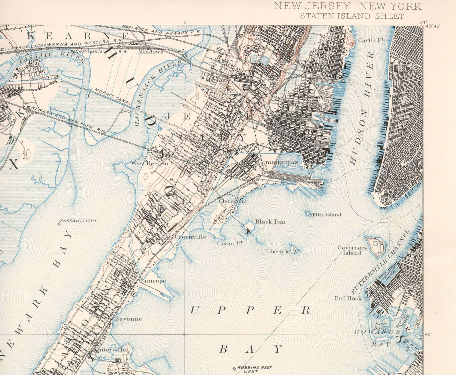
Below are 4 examples of historic USGS quadrangle maps. Figure 3-86 shows the original mapping conducted in 1903 on the 15 minute quadrangle scale, Figure 3-87 shows mapping of La Jolla, California in 1967 on the 7.5 minute quadrangle scale. Figures 3-88 and 3-89 show famous location, Washington, DC (US Capitol area, 1968) and New York Harbor (1891). |

Fig. 3-86. The La Jolla 15 Minute Quadrangle mapped by the USGS in 1903. |

Fig. 3-87. The La Jolla 7.5 Minute Quadrangle mapped by the USGS in 1967. |
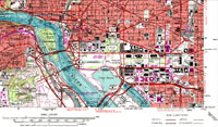
Fig. 3-88. Southwest corner of the Washington DC 7.5 minute quadrangle map of 1968 showing locations where most of the government building and monuments are located near the US Capitol. |
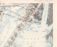 Fig. 3-89. Northwest corner of the Staten Island 15 Minute Quadrangle mapped by the USGS in 1891 showing New York Harbor, parts of Brooklyn and Manhattan. Fig. 3-89. Northwest corner of the Staten Island 15 Minute Quadrangle mapped by the USGS in 1891 showing New York Harbor, parts of Brooklyn and Manhattan. |
|
3.40
Maps Evolved in the Digital Era
In the world of mapping, everything has change. It the days before computers, the mapping of an area of a single topographic 7.5 minute quadrangle took a crew of men (women weren't allowed!) several months to map, and the quality of the work was hindered by rough terrain, bad weather, and often, alcohol and other disputes among men. Despite the problem, the country was mapped, and urban areas were often remapped over-and-over as development progressed. Starting in the 1980s and especially in the 1990s, new methods of mapping evolved that relied on converting imagery from satellites and air-born photography and radar that could create digital geographic data in an instant that would have previously taken months or years, with much more reliable accuracy. It is important to emphasize that the old maps still remain incredibly important! Old maps preserve the history of a region, giving us a glimpse of how the landscape has changes (Figures 3-86 and 3-87 illustrate this for La Jolla, California). It is extremely important for future generations to preserve a history of land use for many reasons, particularly related to environmental health and quality, such as related to water quality issues, location of hazardous waste sites, landfills, and geologic hazard mitigation.
|
3.41
Geographic Information Systems (GIS)
Geographic Information Systems have, arguably, been one of the most important applications of computer technology of our modern era. Maps, and particularly map data provide essential information to nearly all decision making in politics, military, business, agriculture, and social and physical sciences! A GIS (geographic Information system) is a computer application used for capturing, storing, editing, and displaying data related to locations or areas on Earth’s surface. GIS can show many different kinds of data as viewable layers that can be merged on one map, showing features such as streets, streams and lakes, buildings, vegetation, political boundaries, demographic data, and geologic maps. GIS makes it easy to see, analyze, and understand patterns and relationships on a landscape (Figure 3-90).
Two important aspects of modern mapping related to: 1) raw data, and 2) interpretation data.
Raw data is data directly taken from a sensor, such a special type of video camera or radar antenna on a satellite. Raw data include aerial photography, satellite imagery, radar images, or other special sensors able to detect different wavelengths of electromagnetic radiation (such as microwaves, infrared rays, or Xrays), or subatomic radiation. This data can now be processed in real-time and projected in referenced with GPS position data. Old maps, elevation data, and aerial photographic imagery have been digitized and converted into data that can be incorporated as layers in a database for geographic information systems.
Interpretation data is data that comes from other information collection methods. Classic examples include database collections of census data, business sales and financial data, disease and health data, biological resource data, weather and climate data, earthquake data, transportation data... the list can go on and on! Unfortunately, interpretation data can be very subjective, often incomplete, and easily misinterpreted.
|
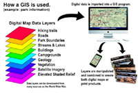
Fig. 3-90. How GIS is used to create maps from raw and interpreted data downloaded from the World Wide Web. |
3.42
Examples of GIS Projections of Using Map Data
DEMs and DOQs are commonly used types of digital map data that show topography natural landscape features, and can integrated into geographic information systems (GIS).
A digital elevation model (DEM) is a raw representation of ground surface topography or terrain (elevation). For example, Figure 3-92 is a DEM of Mount St. Helens area. DEM data is commonly used as a base map in a geographic information systems (GIS). DEMs are created from historic topographic map contour data, or possibly more accurately, from airborne radar data. Each pixel of a computer-generated image using DEM data is assigned with elevation information that can be generate 3-dimensional map view. A DEM can be used for the generation of contours, shaded relief maps, 3-dimensional terrain models. and elevation profiles for cross sections combined with other data.
A shaded relief map is a map of an area whose relief is made to appear three-dimensions using gray-scale shading based on a hypothetical sun angle—such as on a typical late afternoon. Sunshading on a relief map gives a natural appearance that the human eyes and brains can easily interpret. For example in Figure 3-93, sunshading on a digital map of Mount St. Helens makes north and east facing slopes appear darker than south and west facing slopes.
A digital orthoquad (DOQ) is an aerial view a map generated from raw satellite imagery or photography taken from an aircraft that has been digitally rectified to match a latitude-longitude grid associated with a standardize map grid, such as a USGS 7.5 minute quadrangle. Figure 3-94 is an example of DOQ imagery for Mount St. Helens. Satellite imagery associated with Google Maps and other similar platforms are examples of digital orthoquad data. |
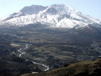
Fig. 3-91. Photograph of Mount St. Helens, Washington. Standard photographs are useful in providing timestamps referenced to landscapes, but they are less important for analyzing data compared with digital map data. The precise time and location of the photograph should be recorded. |

Fig. 3-92. Example of raw DEM data: Digital elevation model of Mount St. Helens, Washington. Note that a DEM shows relief only in a vertical orientation, in 256 shades of gray. It is only raster elevation data and does not show geographic names, roads, etc. like topographic map data. |
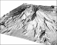
Fig. 3-93. A Shaded relief model for Mount St. Helens, Washington made with DEM data. This image was created with projection enhancement software within a geographic information system (GIS) by processing and re projecting elevation data with sun shading—using the same raw DEM data used to create the image in Figure 3-90. |
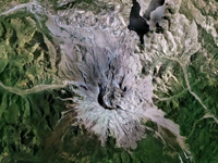
Fig. 3-94. Digital orthoquad [DOQ]) are photographs (images) taken from airplanes or satellites that have been reformatted to precisely match latitude and longitude of landscape features. This is a DOQ of Mount St. Helens, Washington. DOQs are commonly used as base maps—for referencing other data layers in a GIS database. |
|
3.43
The Digital-Dominated Map World
Although there are many map information resources available through the World Wide Web, the mapping platforms provided by Google.com are perhaps the most widely used, and for many good reasons. In addition to their own resources, Google has made map data, databases, and intellectual content available in collaboration with many organizations (government and private), and Google provides a digital platform and public access to a multitude of map-related resources.
Google Earth is an example interactive geographic information system (requires software download). Many kinds of information linked to a database containing geographic reference data can be imported into Google Earth.
Google Maps provides world-wide map information of basic geography (roads, towns, parks, water, landscape features) or on satellite imagery.
ESRI is a corporation supporting the most widely used map editing software (ArcGIS) used widely in industry, education, and government.
The US Geological Survey is a source for many kinds of digital data, including topographic, geologic, water, and maps with other themes.
USGS Map Locater & Down Loader (a source for "free" digital topographic maps on several scales for most of the United States)
USGS National Map Viewer (free online access to digital topographic maps)
See the USGS Maps, Imagery, and Publications (a website to download free digital maps, publications, and imagery)
|

Fig. 3-95. Click on this image to go to the Google Earth information and application download website. |
3.44
KML Files for Google Earth
Many organizations have compiled data for easy import and viewing in Google Earth. The data is in the format of a KML file—a .kml file is geographic information stored in a file format that can be imported into an Earth browser, like Google Earth. KML joins geographic information, (nested elements, such as points, lines, polygons, or 3-dimentional forms) with descriptive information an attributes that allow information to be overlain on the base imagery or maps provided by an Earth browser. Examples of data stored in KML include earthquake and fault information, roads, buildings, flood and fire information, distribution of disease cases, political data—or just about anything that can be visualize on a landscape. KML files can be downloaded from websites and imported into Google Earth. Google Earth provides many data sets (see examples the menu list on the left side of Figure 3-96). |
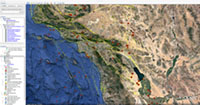 Fig. 3-96. Example of a Google Earth view of the southern California region with a KMLs layer added that show the location of mapped faults, historic earthquakes, and volcanoes. Many more data sets can be turned on or off while exploring regions on Google Earth. Fig. 3-96. Example of a Google Earth view of the southern California region with a KMLs layer added that show the location of mapped faults, historic earthquakes, and volcanoes. Many more data sets can be turned on or off while exploring regions on Google Earth. |
Examples of data in KLM formats
USGS Earthquake Hazards Program - Google Earth/KML Files
https://earthquake.usgs.gov/learn/kml.php
This website provides KML information about real-time earthquakes, mapped locations and history of known earthquake faults, tectonic plate boundaries, geologic maps of the San Francisco Bay region.
National Weather Service - National Weather Data in KML/KMZ formats
http://www.nws.noaa.gov/gis/kmlpage.htm
|
3.45
The discussion below in an introduction to geologic maps, with an introduction landscape features associated with regions around North America.
The links between the traditional landscape studies and mapping of geography and geology intersect in the science of geomorphology.
Geomorphology
Geomorphology is the study of the Earth's surface including classification, description, nature, origin, and development of landforms and their relationships to underlying structures and the history of geologic changes as recorded by these surface features.
Primary studies of landscapes involve generating map of many kinds, including natural landscape features (such as rivers, mountains, shorelines), man-made features (cities, roads, dams, etc.), ecology and land use (natural and agricultural) and much more. Regions of the North American landscape have been subdivided (and classified in some measure) in to regions called physiographic provinces. A physiographic province is a region that has distinct landforms and subregions with shared physical characteristics, such as topography (relief), geologic history, ecology, and climate. Physiographic provinces may display distinct landforms associated with subsurface rock types of common geologic origin, or structural elements. Physiography provinces may have significance to political boundaries, but they can encompass or cut across state and country borders, or political districts.
Physiographic provinces stand out on a shaded relief map of the United States when you compare the topography with regional geology (Figures 3-97 to 3-100).
|
Comparison of shaded-relief map with physiographic provinces and geologic map of the conterminous United States
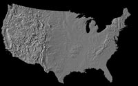 |
 |
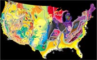 |
 |
Fig. 3-97. Shaded relief map
highlights mountainous regions of the United States |
Fig. 3-98. Physiographic provinces map of the United States |
Fig. 3-99. Physiographic provinces shown on a geologic map of the United States
|
Fig. 3-100. Blank physiographic provinces map of the United States |
|
3.46
|
This website provides an overview of all the physiographic provinces of the United States. Examples of maps, photography, and discussions highlight aspects about each of the physiographic provinces and subregions of the United States. |
3.47
What is a Geologic Map?
A geologic map is a special-purpose map made to show geological features. Types and ages of rock units are shown by color or symbols to indicate where they are exposed at or near the surface. A geologic map records the distribution, nature, and age relationships of rock units and the occurrence of structural features (such as the location of faults). Geologic features are illustrated as colors, lines and symbols.
Geologic maps depict the land as if all soil and vegetation were stripped away. Geologic maps show bedrock characteristics (geologic materials and features), and may display shallow surface sediments (alluvium, landslide deposits, floodplain deposits, sand dunes, etc.). Colors on a geologic map are linked to areas where the bedrock in a region consist rock formations of similar geologic age and composition (example Figure 3-101; the same colors are used for cross sections associated with the map, Figure 3-102). Lines on a geologic map are used to indicate boundaries between rock formations or rocks of different ages, fault lines, and symbology associated with structural features (discussed in Chapter 6).
|
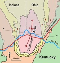
Fig. 3-101. Geologic map of the Cincinnati Arch, Ohio, Kentucky, and Indiana
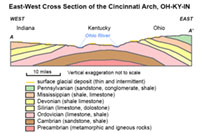
Fig. 3-102. Cross section of the Cincinnati Arch, OH-KY-IN (See A to A' above on Fig. 3-101). |
Fig. 3-101. General geologic map of the Cincinnati Arch region, Ohio, Kentucky, Indiana. This is a fairly simple region to illustrate geologic mapping. The colors on the map show where rocks of different geologic ages occur in the region know as the Cincinnati Arch. The blue line is the Ohio River. A red line defines the glacial boundary (glaciers covered the region during the last ice age north of the red line; when the glacier melted it left behind thin glacial debris deposits on the surface. The red lines with arrow points and small red dip symbols indicate which way the sedimentary strata is dipping gently away from the crest of the structural arch.
Figure 3-102. East-West Cross Section of the Cincinnati Arch, Ohio, Kentucky, Indiana. The cross section is made along the line between the letters A and A' on Figure 3-101. The cross section shows the general geologic arrangement of layers below the surface across the region. |
| Geologic maps are used to interpret the geologic history of a region. Geologic maps are used by paleontologists to find areas that are likely to contain fossils, and by geologists and engineers to define the location of faults, economic mineral resources, to find potential underground water resources, used in civic planning of infrastructure (placement of power plants, sewer systems, highways, bridges, buildings), and more. |
3.48
Below is a list of essential concepts needed to interpret geologic maps.
Note that some of the concept are addressed in more detail in other chapters. |
geologic time scale and rock types (and rock cycle)
|
strike & dip
faults & folds
(discussed in Chapter 7) |
strata
Law of Superposition
Law of Original Horizontality
Law of Cross-Cutting Relationships
|
unconformities
|
| relative and absolute dating |
surficial deposits (alluvium, soils, landslides, etc.)
(discussed in Chapter 9) |
|
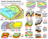
Fig. 3-103. Common symbols representing geologic features on geologic maps. Concepts illustrated describe strike and dip for describing the orientation of strata (beds), and illustrations of structural features (folds and faults). |
Fig. 3-104. Basic geologic principles: laws of original horizontality, superposition, and cross-cutting relationships |
Fig. 3-105. Unconformities: types include nonconformities, disconformities, and angular unconformities. |
3.49
Comparison of a Topographic Map and Aerial Imagery With a Geologic Map
Most of the past geologic mapping conducted in the history of the United States was using topographic maps as the base for interpreting the geology of a landscape. Both topographic maps and geologic maps have been created using aerial photography (when it became available). Geologists needed a basic knowledge of geomorphology and basic geologic principles to create map. Often geologic maps of many areas have been revised as new data became available. Geologic mapping can be very difficult, requiring geologists to try to access very rugged terrain and often hazardous conditions on the ground. In many areas there are no rocks exposed on the surface, and geologist have to make educated guesses as to what exists below the surface. However, new data provides incite for revising geologic maps. New data may include information found on satellite imagery or aerial photography, discovery of previously unknown outcrops, fossils, new dates from absolute dating, or discoveries made during excavations for buildings and infrastructure. Topographic, aerial photograph, and geologic maps are compared for the San Juan Bautista 7.5 minute quadrangle, California in Figures 3-106 to 3-111. |
Comparison of a topographic map with a geologic map
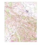 |
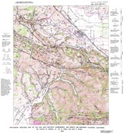 |
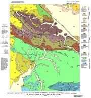 |
Fig. 3-106. Topographic Map of the San Juan Bautista, California
15 minute quadrangle |
Fig. 3-107. Topographic map with geology line mapping (shown on map in Figure 3-106) |
Fig. 3-108. Geologic Map
of the San Juan Bautista, California 15 minute quadrangle |
| Modified from: Dibblee, Thomas, W, 1979, Preliminary Geologic Map of the San Juan Bautista Quadrangle: U.S. Geological Survey Open-File Report 79-375, scale 1:24,000. |
Comparison of a aerial photograph map (DOQ) with a geologic map
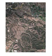 |
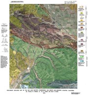 |
|
| Fig. 3-109. Aerial photography covering the San Juan Bautista, CA 15 minute quadrangle |
Fig. 3-110. Geologic data superimposed on aerial photography (shown on map in Figure 3-108) |
Fig. 3-111. Geologic Map
of the San Juan Bautista, California 15 minute quadrangle |
|
3.50
Interpreting the Earth structure with maps and geologic illustrations
Geologic Maps, cross sections, and block diagrams are used to show the structure of the Earth in three dimensions. Geologic maps show the arrangement of geologic features and materials exposed on or near the surface. Cross sections show interpretations of geologic features, structures, and materials in vertical profiles, usually perpendicular to the surface.
Examples below are from part of the Grand Canyon, Arizona area (Figures 3-112 to 3-116).
(The map and associated figures modified from Billingsley, G. H., 2000, Geologic map of the Grand Canyon 30' x 60' quadrangle, Coconino and Mohave Counties, northwestern Arizona: U.S. Geological Survey Geologic Investigations Series I-2688, map scale 1:100,000. http://pubs.usgs.gov/imap/i-2688/). |
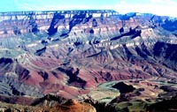
Fig. 3-112. Grand Canyon (photo view is looking north from the South Rim)
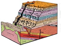 |
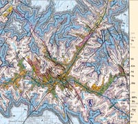 |
 |
Fig. 3-113. Grand Canyon Geologic Map. Line D - D' is the location of the cross section shown below.

|
| Fig. 3-114. Block Diagram of the Grand Canyon |
Fig. 3-115. Geologic Cross Section of the Grand Canyon |
Fig. 3-116. Geologic map legend for the Grand Canyon |
|
3.51
Finding Geologic Map Information
To find a geologic map of portions of the United State it is usually essential to find the name of the topographic map name of a particular region. The USGS typically names small scale geologic maps with the name of the 7.5 minute topographic map quadrangle (1:24,000 scale). Larger scale (regional maps) are named after the 1:100,000 maps (1° x 2° quadrangle) or larger 1:250,000 scale. State geologic maps are typically 1:1,000,000 scale or larger.
Geologic maps can be located using the National Geologic Map Database: http://ngmdb.usgs.gov/ngmdb/ngmdb_home.html
The National Geologic Map Database provides access to maps in digital formats and bibliographic information for maps published in paper formats that might be located in library map collections or purchased from the US Geological Survey and state geological surveys. Unfortunately accessing paper map collections is becoming increasingly difficult because the high cost of maintaining these antiquated collections.
|
Important additional resources for interpreting geologic maps
FGDC Digital Cartographic Standard for Geologic Map Symbolization
http://ngmdb.usgs.gov/fgdc_gds/geolsymstd/download.php
Symbols Used On Geological Maps
http://www.ga.gov.au/image_cache/GA17066.pdf |
3.52
3.54
Answer to the Cross Section Exercise in Figure 3-45.
The
order of formation (from oldest to youngest) is: P - E - F - D - I - L - O - M - J - H - A - K- G - N - B - C
Note that it is sometime easiest to start at the top and work backward on such diagram before you recreate the "geologic history" of an cross section. Here is what happened here (starting from oldest to youngest).
Sedimentary layers were deposited (following the Laws of Superposition and Original Horizontality).
1. P — shaly sandstone was deposited as a horizontal layer.
2. E — mudstone was deposited as a horizontal layer.
3. F — layers of sandstone were deposited as horizontal layers.
4. D — more mudstone and shaly sandstone layers were deposited as horizontal layers.
5. I — represents a fault that formed during a period of mountain building where the older layers P, E, F, and D were folded, faulted and intruded by igneous rock.
----- The law of cross-cutting relationships depicts that the fault [ I ] is younger than sedimentary layers P ,E, F, and D.
6. L — represents an unconformity, mountain building had ended, the landscape had eroded flat over a long period of time.
7. O — sandstone was deposited as a horizontal layer on top of the ancient eroded landscape surface.
8. M — shale was deposited as a horizontal layer on top of the sandstone [M].
9. J — layers of limestone were deposited as horizontal layers on top of the shale [J].
10. H — a fault formed, cutting through all the previously formed rock layers - as defined by the law of cross-cutting relationships.
11. A — the letter A represents an unconformity - layers of limestone on the right side are thinner, suggesting there was either erosion and/or non-deposition.
12. K — a layer of sandstone was deposited above the unconformable surface.
13. G — a layer of shale was deposited on top of the sandstone.
14. N — an igneous intrusion cut through all previously formed rock units, possibly forming a volcano.
15. B — after the igneous intrusion {N] formed, erosion stripped away any evidence of a possible volcano, and a layer of sandstone [B] was deposited.
16. C — another igneous intrusion formed, resulting in eruptions that formed the volcano still present on the land's surface.
Other things to consider on this cross section exercise.
Note the igneous rocks with X markings on the right side of the diagram are truncated by the unconformity [L] - the same as the fault [ I ]. Which one is older? It is impossible to tell — they are "relatively" the same age. In addition, all the boundaries between the rock formations could be unconformities, but their significance in age differences would have to be determined by some other means.
Unconformity [L] clearly demonstrates that it is an unconformity represents a long period of time passage. In some places it is an angular unconformity; over the intrusion [ with the X markings] it is a nonconformity.
The unconformity marked as letter A is somewhat problematic. It truncates the fault (letter H). The problem is that it would take further examination to determine whether or not fault H was forming at the same time that limestone J was being deposited!
The boundary between sedimentary layers G and B is also an unconformity that represents a significant passage of time — at least long enough for a volcano to form and then be stripped away by erosion.
|
|