
Oceanography 101 |
Return to class home page |
Chapter 9 - Ocean Circulation |
The Atmosphere and Ocean Circulation Systems Are Linked |
Click on thumbnail images for a larger view. |
| The global atmospheric circulation system influences the movement of air masses in general "belts" that move air in rotating masses within zones around the planet (Figure 9-1). These relatively stationary wind belts impact the surface of the oceans, creating currents that circulate waters in the oceans under the influence of Coriolis effect, creating five large subtropical gyres encircling the major oceans basins (Figure 9-2). Currents in the oceans include surface currents and deep currents: • surface currents are driven horizontally by effects of the wind. • deep currents are driven horizontally and vertically by differences in density (density changes typically start near the surface). Ocean circulation is also influenced by seawater temperature and density. • Warm water in the tropics flows in currents to polar regions where it cools and the formation of sea ice concentrates the salt in seawater, increasing its density so that it sinks. • Cold and salty water (concentrated by surface evaporation) sinks. Elsewhere seawater rises where it is displaced by colder and saltier water. |
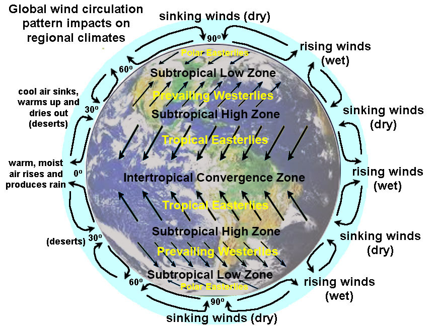 Fig. 9-1. Global wind circulation patterns impact regional climates and drive the large surface currents in the global ocean circulation system. |
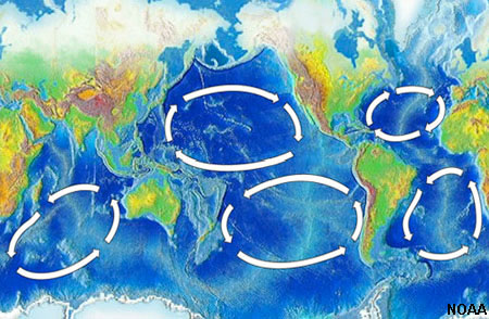 Fig. 9-2. Five large gyres circulate surface waters in the global oceans. These rotating subtropical gyres are influenced by the patterns of atmospheric winds and the Coriolis effect. |
Deep-Ocean Thermohaline CirculationOcean circulation is also influenced by seawater temperature and density. Cold and salty water (concentrated by surface evaporation) sinks. Elsewhere seawater rises where it is displaced by colder and saltier (denser) water (Figure 15-20). Warm water in the tropics flows in currents to polar regions where it cools. In the Arctic region, the formation of sea ice concentrates the salt in seawater, increasing its density so that it sinks. Cold, salty water sinks both in the Arctic and Antarctic regions, feeding deep ocean circulation. The differences in temperature and salinity (or overall density) is the driving force behind deep-ocean thermohaline circulation (Figure 15-21). The coldest and densest (saltiest) water form around Antarctica where massive amount of sea ice forms. When seawater freezes, the sea ice is salt free (expelling the salt). The expelled salt adds to the saltiness (and density) of the coastal waters around Antarctica, causing them to sink in a slow current into the deep ocean basins. Lesser amounts of sea ice form in the northern Arctic region and around Greenland.The deep ocean basins have slow moving currents (compared with the surface waters exposed to atmospheric winds. As currents move about the globe, evaporation increases salinity. Increased salinity combined with cooling increases seawater density, allowing affected seawater to sink into the deep ocean. The movement of surface waters downward supplies oxygen to the seabed, assisting in the decay of organic matter. The deep, slow-moving water picks up nutrients from the seafloor and from decaying organic particles sinking through the water column. In locations where deep-water upwells to the surface, these nutrients supply the ingredients for phytoplankton blooms, providing food for the food chain.
|
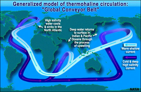 Fig. 9-3. Thermohaline Circulation: cold and salty ocean water is dense and sinks. Warm water stays at the surface. Evaporation increasing salinity (and increasing density) before it can sink. Formation of sea ice also increases salinity. 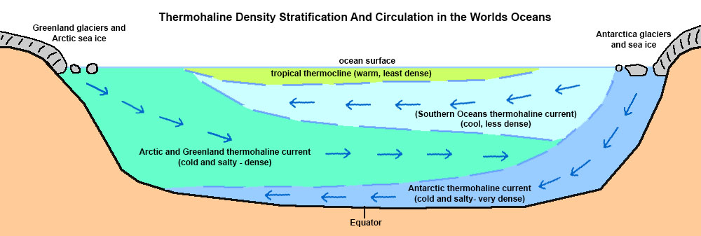 Fig. 9-4. Thermohaline density stratification and currents of the world's oceans. |
Sea Ice and Thermohaline CirculationGlaciers flowing into the ocean contribute large amounts of iceberg and sea ice to the polar ocean regions. However, sea ice also forms where very cold air is in contact with the ocean surface. Currents in the upper sea (mixing zone) can inhibit the formation of sea ice. Water is most dense slightly above the freezing point and tends to sink whereas ice floats. Once sea ice starts to form the salt is either expelled back into the seawater and some is concentrated in microscopic pockets trapped in the sea ice. Antarctic sea ice is typically 1 to 2 meters (3 to 6 feet) whereas most of sea ice in the Arctic is 2 to 3 meters (6 to 9 feet) thick. However, in some Arctic regions sea ice can grow to 4 to 5 meters (12 to 15 feet) thick. The formation of sea increases the salinity of the seawater, and the combination of the increased salinity and cold water results in the formation of dense water that sinks into the deep ocean, driving the thermohaline circulation through the world’s deep ocean basins.Arctic Sea Ice time lapse from 1987-2009 (NOAA/NSIDC satellite data YouTube video) |
 Fig 9-5. Origin of glaciers, icebergs, and sea ice. Sheets of sea ice form and melt back with the seasons. |
Surface CurrentsSurface Currents involve large masses of water moving horizontally on the surface.• The transfer of wind energy to water is not very efficient (only about 2% energy transfer of “friction” between water and air). • Wind produces both waves and currents (more on waves in Chapter 10). • Surface currents occur in the mixing zone within and above the pycnocline (layer of rapidly changing density). • Effects of surface currents is to redistribute heat from equatorial to polar regions. |
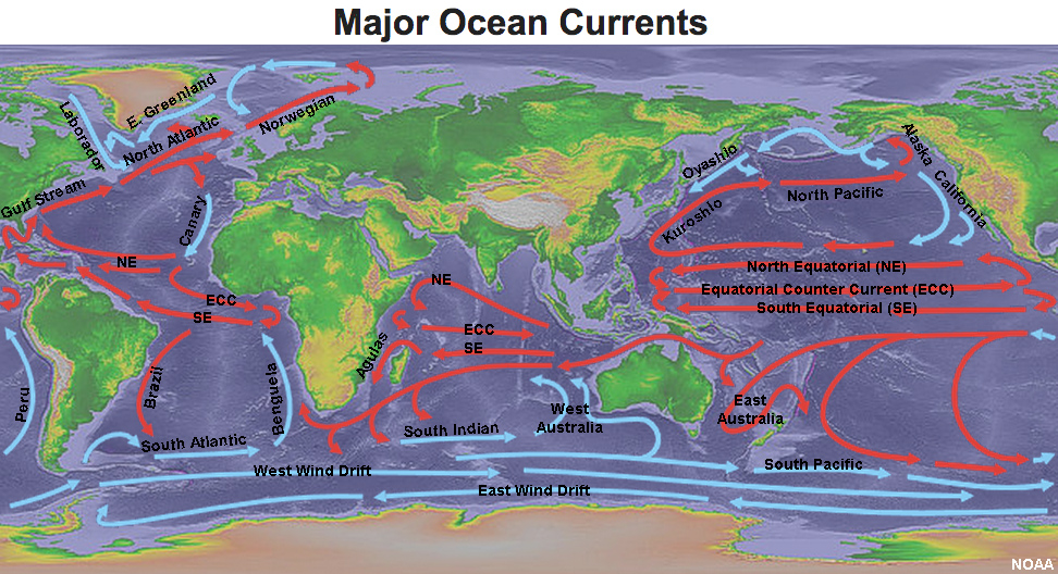 Fig. 9-6. Major surface currents of the oceans. |
| Mechanisms moving surface currents include: • Wind: major mechanism (result of atmospheric circulation patterns). • Solar heating: (direct heating by the sun) - a minor mechanism (influences surface waters but not water at depth). • Tides: (affect currents in coastal regions - tidal currents are discussed in Chapter 10). • Geography: locations of continents (and islands) influence direction and flow currents (acting as barriers to flow). Subtropical gyres are large system of rotating ocean surface currents driven by global wind currents with the influence of Ekman Transport (see below) and continental geography (land masses restrict and deflect the flow of water currents). |
Movement of Surface CurrentsMoving water (like wind) are influenced by the Coriolis effect (Figure 9-7):• Moving water is deflected to the RIGHT in the Northern Hemisphere. • Moving water is deflected to the LEFT in the Southern Hemisphere. The Coriolis effect has a large influence on the movement of both surface water and deeper water. However, wind-driven currents move fastest near the ocean surface and diminish with depth. The difference in rate of movement results in a rotational process called Ekman transport. |
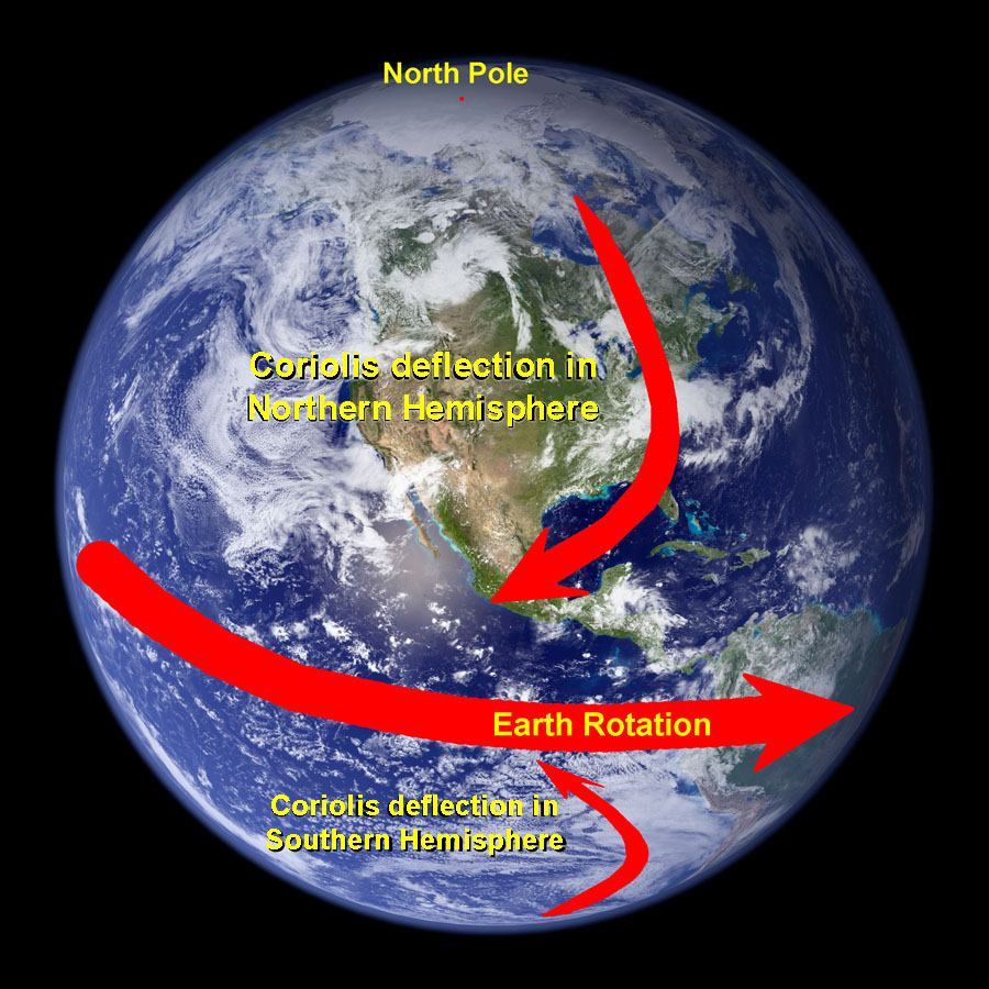 Fig. 9-7. Coriolis effect. |
Ekman Spiral and Ekman TransportEarly sailors traveling in regions where icebergs are common noticed that the icebergs moved in a different direction than the wind (causing alarm as the icebergs were cutting across the paths of ships moving down wind).Walfrid Ekman (1874-1954, a Swedish physicist) resolved the problem of why wind currents and water currents were not the same. The force of wind affect surface water molecules, which in turn, drag deeper layers of water molecules below them (drag is caused by friction between water molecules). The deeper below the surface, the slower the water moves compared to the water layer above it. Surface movement ceases at a depth of about 100 meters (330 feet). As noted above, both surface water and deeper water is deflected by the Coriolis effect. —90° to the right in the Northern Hemisphere —90° to the left in the Southern Hemisphere. Depth is important: Each successively deeper layer of water moves more slowly to the right (or left), creating a spiral effect (called the Ekman Spiral). Because the deeper layers of water move more slowly than the shallower layers, they tend to twist around and flow opposite to the surface current. Net result is that net transport in surface currents is 90° from wind (Figure 9-9). This twisting character of ocean surface waters is called the Ekman spiral. The impact of the Ekman Spiral is enhanced where geographic features create barriers to the movement of water. Ekman transport is the net motion of a fluid (seawater) as the result of a balance between the Coriolis effect and turbulent drag forces (within surface waters and geographic features (shoreline and seabed). |
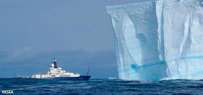 Fig. 9-8. Sailors of ships noticed that icebergs move in a different direction than the wind. 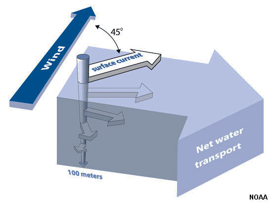 Fig. 9-9. The Ekman spiral |
Ocean CurrentsOcean Surface Speed video: This sea surface temperature (SST) simulation from a NOAA high resolution coupled atmosphere-ocean model. The video shows ocean currents speed and behavior based on sea-surface temperature data. As the animation focuses on various locations of the world ocean we see the major current systems, such as the Agulhas current, Brazil current, Gulf Stream, Pacific Equatorial current, Kuroshio current. The small scale eddy structure is resolved and evident. This simulation is from the NOAA's Geophysical Fluid Dynamics Laboratory. |
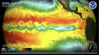 Click on image to start video. |
Boundary CurrentsBoundary currents currents associated with gyres flow around the periphery of an ocean basin.• Boundary currents are ocean currents with dynamics determined by the presence of a coastline. Two distinct categories of boundary currents: • western boundary currents • eastern boundary currents. |
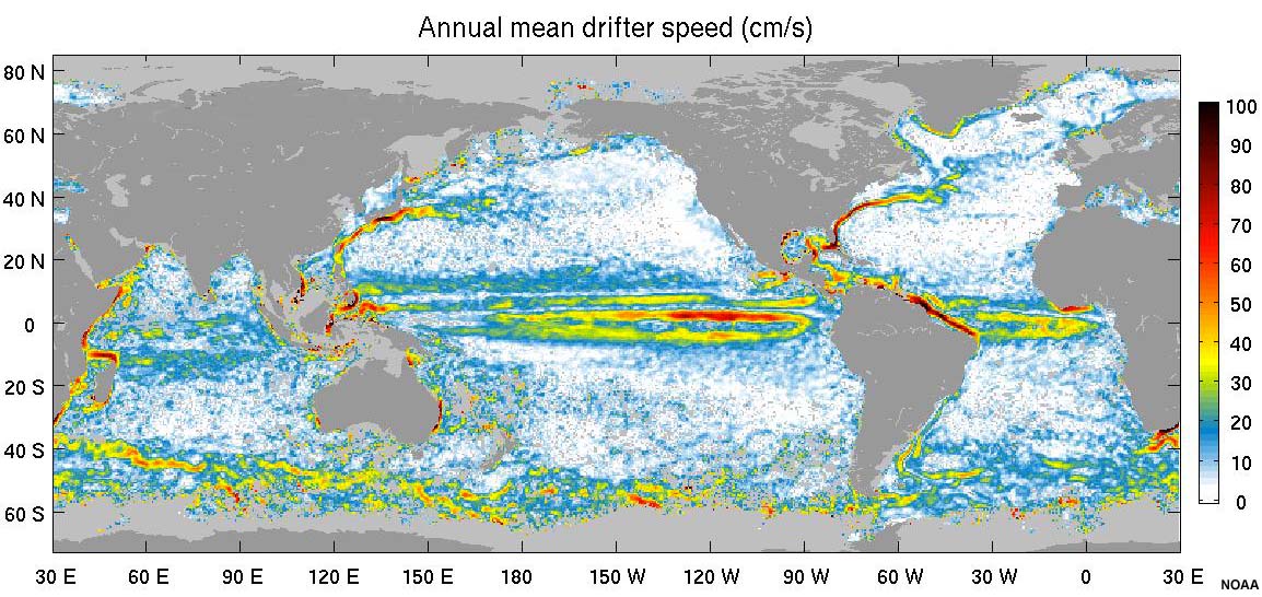 Fig. 9-10. Speed of currents measured by drifting devices (annual average in cm/sec) |
Western Intensification of Boundary CurrentsWind blows westward along the inter tropical convergence zone at the equator, causing western intensification.• Wind blowing across the oceans mounds water on the western side of ocean basins-up to 2 meters. • The mounding of water is caused by converging equatorial flow and surface winds. • The Coriolis effect is most intense in polar regions, so current flowing eastward near the poles is more dissipated than currents flowing westward at the equator. • The higher side of a mound is on the western side of the ocean basins, having a steeper slope and therefore faster moving. Eastern boundary currents are slow (a few miles or km per day), wide (less than 600 miles [1000 km]), and shallow (less than .3 miles [.51 km]). Examples include the Canary, California, Benguela, and Peru currents (see Figures 9-10 and 9-11). Eastern boundary currents form along the cool and dry east side of ocean basins. Western boundary currents (WBC) are fast (many miles or km per day), narrow (less than 60 miles [100 km] wide), and deep (up to 1.3 miles [2 km]) Examples include the Gulf Stream, Brazil, Kuroshio, East Australian,and Agulhas currents (see Figures 9-10 and 9-11). Western boundary currents form along the warm and wet west side of ocean basins. |
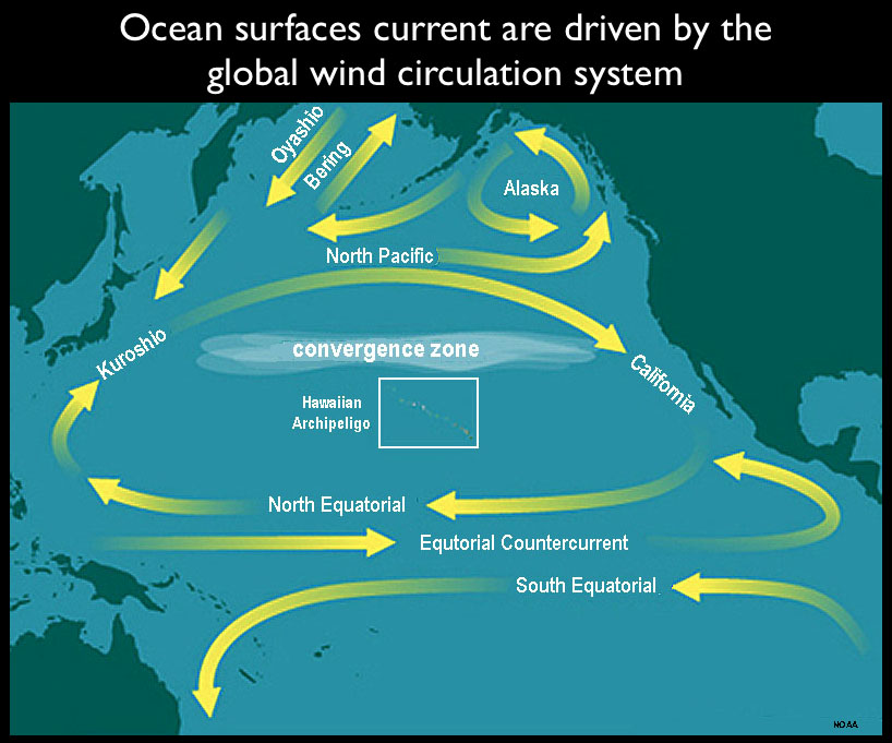 Fig. 9-11. The California Current is an eastern boundary current; part of the Northern Pacific Gyre. The Kuroshio Current near Japan is a western boundary current. |
| Gyres and boundary currents are large scale features, but are also complex. Boundary currents change constantly (called meandering) producing spinning cone-shaped masses of water—spinning off of the larger boundary currents. Eddy CurrentsMeandering currents produce eddies. Satellite temperature data of the ocean surface reveals the spreading and mixing of surface waters as currents move from one region to another, gaining intensity and dispersing energy as they move. The temperature data reveals large spinning eddies in portions of the ocean basins along the margins of major currents.Figure 9-12 illustrates large eddy currents forming in the surface waters of the southern Atlantic Ocean west of southern Africa as revealed by satellite ocean surface temperature data. The eddy currents form as a part of the meandering processes that dissipate energy in the ocean waters. This meandering creates warm- and cold-core rings of swirling currents (Figure 9-13). |
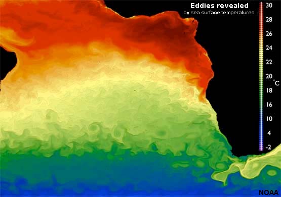 Fig. 9-12. Large eddy currents in the South Atlantic Ocean revealed by surface temperature data. |
Warm-Core Rings and Cold-Core Rings• Warm-core rings are rotating warm masses of water surrounded by colder water. Example: Warm water areas in the Sargasso Sea water surrounded by cool water (Figure 9-14).• Cold-core rings are cold masses of water surrounded by warmer water. These spinning rings can last for years and serve as refuges for sea life (warm and cold water) and can influence storm development (such as intensifying or reducing hurricane intensity). Core rings typically have unique biological populations. Cold-core rings are locations where upwelling takes place, resulting in more biological productivity. Core rings can form and last for months and migrate with currents across ocean basins. |
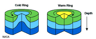 Fig. 9-13. Warm- and cold- core rings are created by eddies in ocean currents (Northern Hemisphere examples). |
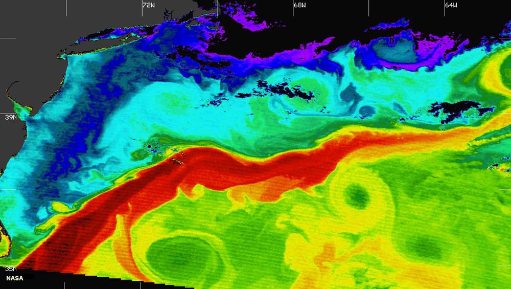 Fig. 9-14. Cold-core rings (shown with green centers in these thermal satellite images) in the North Atlantic are associated with the Gulf Stream current. |
The Gulf Stream CurrentThe Gulf Stream is a fast moving ocean current (Figure 9-15).• The North Equatorial Current moves east across the Atlantic Ocean in the Northern Hemisphere. • This flow splits into the Antilles Current (east of the West Indies) and the Caribbean Current (around the Gulf of Mexico). • These currents merge into the Florida Current. (about 30-50 miles [50-80 km] wide, moving 2-6 mph [3-10 km], and about a mile deep). • Along the East Coast, the Gulf Stream experiences western intensification. • North of Cape Hatteras (NC) the current moves away from the coast and gradually looses much of its intensity (by meandering) producing numerous warm and cold core rings. • The Gulf Stream gradually merges eastward with the water of the Sargasso Sea, the rotating center of the North Atlantic Gyre (named for floating marine alga (seaweed) called Sargassum that accumulates in the stagnant waters. • For comparison, the volume of water moved by the Gulf Stream is about 4 billion cubic feet of water per second, more than all the world's rivers combined! |
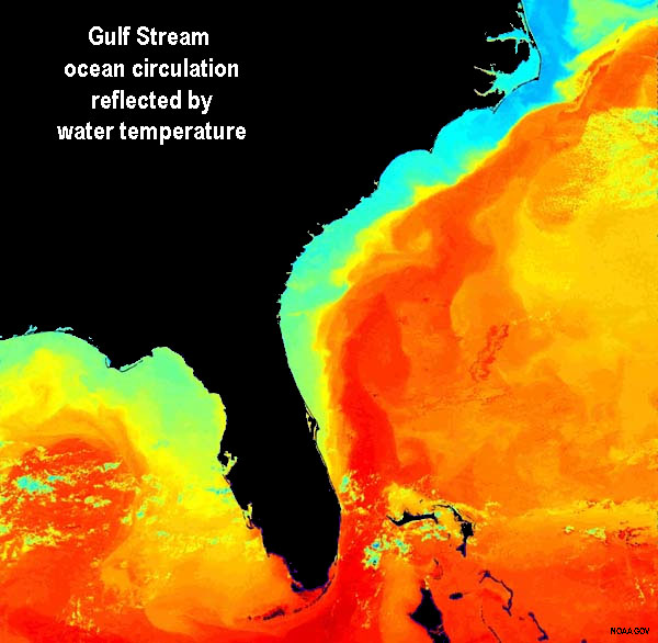 Fig. 9-15. The Gulf Stream is the world's largest ocean current (revealed here by water temperature patterns). |
The Florida Current and the Gulf StreamThis animation focuses on the Florida Current (also known as the Loop Current) as it flows into the Gulf Stream (a major surface current). The Florida Current is a body of warm surface water that travels up from the Caribbean, past the Yucatan Peninsula, and into the Gulf of Mexico, then flows through the Florida Strait, into the Gulf Stream. From there heads north as the Gulf Stream up the eastern coast of the U.S. Note the black colors indicate the warmest ocean surface temperatures and and light blues indicate the coolest temperatures. This sea surface temperature (SST) simulation from the NOAA's Geophysical Fluid Dynamics Laboratory’s. |
 Click on image to start video. |
Antarctic Circumpolar Current• The Antarctic Circumpolar Current is the only current to completely encircle Earth (Figure 9-16).• The current moves more water than any other current. • The current is in a region of the world with intense winds and wave action. • The region has lots of upwelling - very "rich" ocean basin (nutrients for plankton; food for higher-level feeders), See an animation of the changes in the mixing zone depth by seasons: Antarctic Circumpolar Current (NOAA). With stronger circumpolar winter winds (June-August), the wave height increases in the wind belt around Antarctica increases, and the depth of current mixing water increases. This feeds more oxygen and food into deeper water, supporting a rich open-ocean ecosystem. |
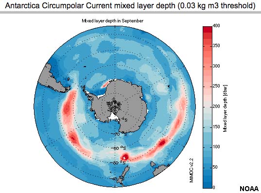 Fig. 9-16. Antarctic circumpolar current revealed by mixing zone depths. |
Arctic Ocean CurrentsThis video show Arctic Ocean currents based on NOAA sea-surface salinity satellite data. This animation shows the seasonal cycle of summertime freshening from sea ice melt as well as the salty water entering from the North Atlantic current. This simulation is from the NOAA's Geophysical Fluid Dynamics Laboratory. |
 Click on image to start video. |
Climate Effects Of Ocean Currents• Cold water offshore results in dry condition on land (example: California).• Warm water offshore results in more humid condition on land (example: Florida). • Depends on seasonal wind patterns and water temperatures. • Depends also on regional geography along coastal regions. |
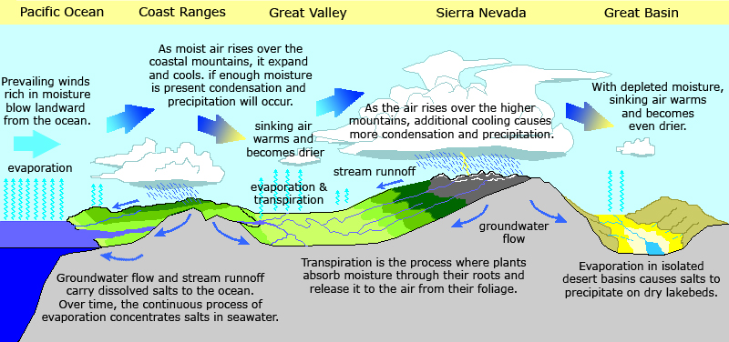 |
| Fig. 9-17. California's climate and geographic factors. |
Upwelling and DownwellingUpwelling is the vertical movement of cold, nutrient-rich water from deep water to the surface, resulting in high productivity (plankton growth).• Can bring cold, nutrient-rich water to the surface (photic zone) unless thermocline is strong and prevents it. • Nutrients are not food but act like a fertilizer. • Upwelling water rich in nutrients feeds phytoplankton, the base of the food chain. Downwelling is the vertical movement of surface water downward in water column. Regions where downwelling is occurring typically have low biological productivity. • Downwelling takes dissolved oxygen down where it is consumed by the decay organic matter. |
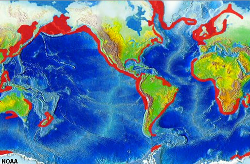 Fig. 9-18. Regions of the world where coastal upwelling occurs. |
Where Upwelling OccursDiverging surface waters occur where surface waters are moving away from an area on the ocean surface. This results in upwelling as deeper water gets moves upward to replace surface waters being moved away by the wind. Two types include:• Equatorial upwelling occurs where SE trade wind blow across the equator (Figure 9-19); Ekman transport forces surface water movement to the south (south of the Equator), and to the north (north of the Equator). Upwelling of deep ocean waters is most intense in equatorial regions. • Coastal upwelling occurs where wind blowing along a coastline is influenced by Ekman current moving surface waters offshore, or winds blowing off the land pull surface waters away from the coast, pulling deeper water up to replace surface waters. See Figure 9-18 for locations where coastal upwelling most commonly occurs. • Other locations where upwelling occurs include around underwater obstructions (guyots) or sharp bends in coastlines. |
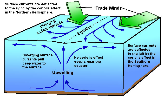 Fig. 9-19. Equatorial upwelling involves the Trade Winds blowing across the equator and the Coriolis effect taking over as diverging currents move away from the equator. |
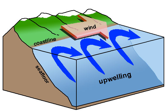
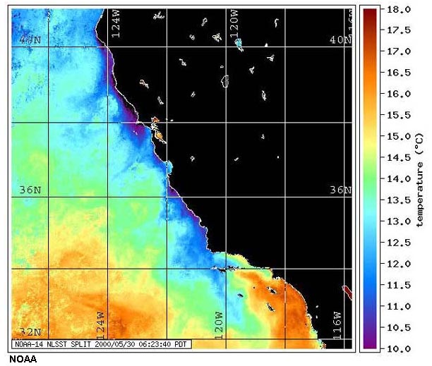
Coastal Upwelling and DownwellingThe continental margins of the world are places where coastal upwelling and downwelling are taking place (Figure 9-18). Coastal upwelling is influenced by coastal geometry, wind directions, and the influence of the Coriolis effect (Ekman transport). Figures 9-20 and 9-21 illustrate how the direction of wind movement determines how coastal upwelling and downwelling takes place in the Northern Hemisphere (such as in California). Figure 9-22 shows regions of coastal upwelling along the California continental margin—revealed ocean-surface temperature imagery. Upwelling water along the coastline is colder than waters farther offshore. |
 |
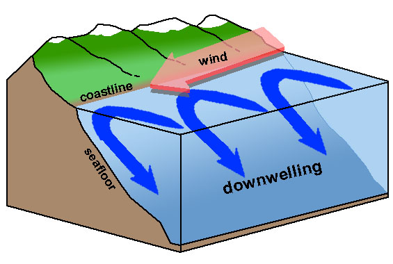 |
| Fig. 9-20. Coastal upwelling (example of California) | Fig. 9-21. Coastal downwelling (wind reversed) |
Large Cycles in Ocean Climate VariabilityThe ocean/atmosphere systems display cyclic changes beyond annual seasonal changes. Longer-term cycles are also taking place. Changes happening in one region can gradually impact other regions on multi-year to decade cycles (example: cycles in coastal upwelling on North America's West Coast, Figure 9-23). Even longer-term cycles are influenced by extraterrestrial pattern changes in the orbit and rotation of the Earth relative to the Sun over time. These changes impact the distribution of precipitation and influence the warming or cooling of climates over multi-year periods, and changes in sea level over time linked to the accumulation and melting of continental glaciers. |
 |
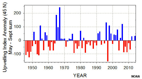 |
| Fig. 9-22. Upwelling offshore of California revealed by ocean surface temperatures. | Fig. 9-23. Cycles of upwelling on North America's West Coast influenced by ENSO. |
El Niño/Southern Oscillation (ENSO)El Niño/Southern Oscillation (ENSO) in the Pacific Ocean [also called El Niño-La Niña Cycles] is associated with a band of warm ocean water that develops in the central and east-central equatorial Pacific. El Niño/Southern Oscillation (ENSO) is perhaps the most important ocean-atmosphere interaction phenomenon to cause cyclic global climate variability. Here's how the ENSO cycle works: ENSO involves the interactions of ocean currents, ocean temperatures, and atmospheric effects, over time.Pacific Ocean Currents Involved With ENSO• West moving winds at the Equator help to drive the two Pacific Subtropical Gyres (northern and southern gyres)(see Figures 9-6).• In the North Pacific Subtropical Gyre, the western-intensified Kuroshio Current moves up the Asian seaboard (warming China, Japan), flows east with the North Pacific Current, then south as the California Current along the west coast of North America. • In the South Pacific Subtropical Gyre, the western intensified East Australian Current moves south and merges with the Antarctic Circumpolar Current, the completes the gyre as the Peru Current (flowing northward along the west coast of South America). ENSO Ocean Temperature EffectsENSO Cycles are influenced by ocean surface temperatures throughout the Equatorial Pacific Ocean region. During the El Niño periods, ocean surface temperatures are much warmer than the La Niña periods. This is a reflection of the amount of cloud cover (deflecting incoming solar radiation) and winds driving cold upwelling currents to the ocean surface in the equatorial region. During El Niño periods, the Pacific Warm Pool grows larger and more intense in the Eastern Pacific region near Australia and Indonesia (Figure 9-24).ENSO Weather Effects And the Walker Cell• The rising warm-moist air in the western Pacific contrasts with the cool sinking air along South America, resulting in the Walker Cell (an unstable equatorial air circulation pattern region in the Pacific Ocean)(Figure 9-25). The Walker Cell operates perpendicular (east to west, not north to south like the Hadley, Farrell, and Polar circulation cells [see Figure 15-15]). the intensity Walker Cell weather pattern is controlled by temperature contrasts on opposite sides of the Pacific Basin along the equator. |
 Fig. 9-24. Ocean surface temperatures reveal the changing patterns and regional extent of the Pacific warm pool associated with El Niño-La Niña Cycles. 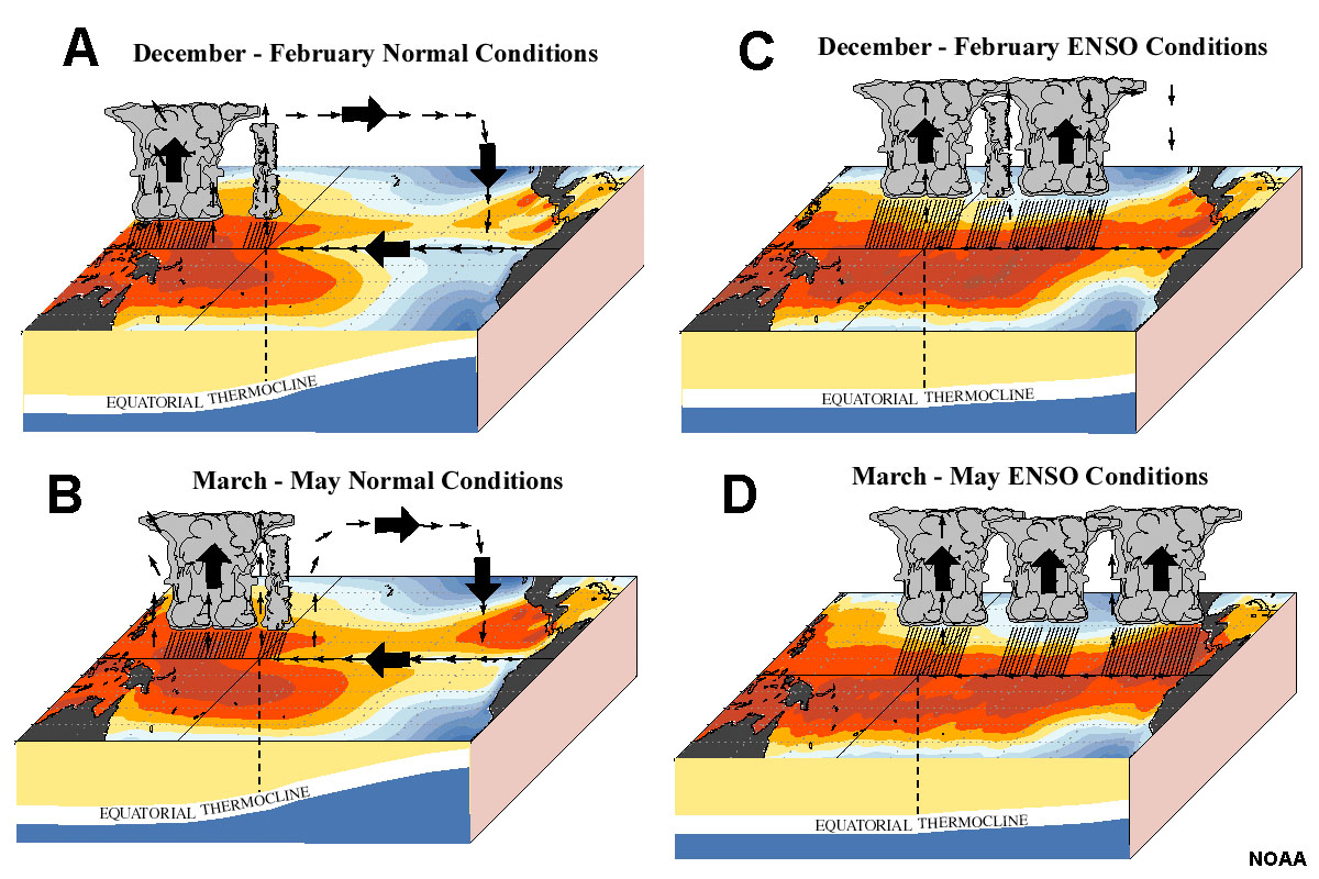 Fig. 9-25. El Niño-La Niña Cycles changes in the Walker Cell wind currents affect ocean surface temperatures which impact the thickness and extent of the thermocline (which impacts upwelling). |
|
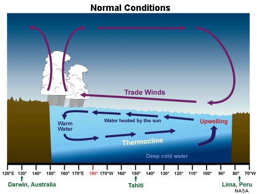
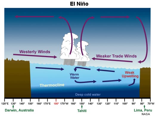
Under normal year ENSO conditions (which is actually rare) cool water conditions persist along the west coast of South America (Peru) (Figure 9-26): • Trade winds blow to the west allow waters to upwell along the west coast of South America (some of the most productive waters in the world). • West-moving winds drive surface currents westward across the Pacific Ocean where they heat up creating the Pacific Warm Pool - a thick thermocline in the western Pacific Ocean. Under El Niño (the warm phase of ENSO) wind intensity of the Walker Cell circulation is diminished (Figure 9-27). El Niño is associated with high air pressure in the western Pacific and low air pressure in the eastern Pacific. La Niña (the cool phase of ENSO) is associated with below average surface water temperatures and high air pressures in the eastern Pacific and low air pressures in western Pacific (Figure 9-28). Air circulation in the Walker Cell is intensified. |
 |
 |
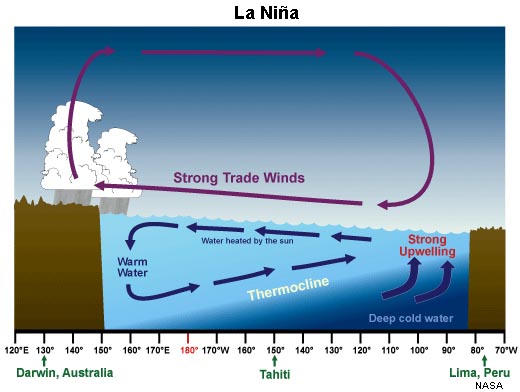 |
| Fig. 9-26. A normal year thermocline and weather pattern under somewhat rare normal conditions in the equatorial Pacific region. | Fig. 9-27. El Niño thermocline and weather during strong El Niño conditions in the equatorial Pacific region; coastal upwelling near South America is diminished. | Fig. 9-28. La Niña thermocline and weather during La Niña conditions in the equatorial Pacific region; coastal upwelling near South America is strengthened. |
|
| El Niño/La Niña Global Climate Impacts—NOAA videos, websites, animations El Niño/La Niña Explained (YouTube video). NOAA's El Niño website. El Niño/La Niña 1997-1998 (NOAA) - Shows sea surface temperature time lapse. Global Sea Surface Temperature time lapse showing El Niño/La Niña (NOAA) |
|||
| El Niño Simulation: This animation of model output illustrates the three dimensional complexity which is resolved in this model. A section of the Equatorial Pacific is showcased as it evolves through several ENSO events. The surface temperature are daily output while the subsurface temperatures are interpolated from monthly output. Salient features are the tropical instability waves and their subsurface impact, the evolution of the tropical thermocline through the events and the impacts of the presence of a well represented Galapagos Archipelago. |  Click on image to start video. |
Impacts of ENSO CyclesENSO cycles [El Niño-La Niña Cycles] consist of shifting weather and oceanographic conditions in the tropical Pacific region (refer to Figures 9-24 and 9-25).During El Niño:• High and low atmospheric pressures systems reverse across the equatorial Pacific region. As a result the Walker Cell circulation pattern is very weak.• Winds become slack or blow against the west-moving Equatorial Current. • The west-moving Equatorial Current mounds warm water on eastern side of Pacific Basin. near Australia and Indonesia. • Along the coast of South America, a normally thin temperate thermocline replaced with a thick tropical thermocline. • This thick thermocline prevents mixing of deep cold nutrient rich water because of the buoyancy of extra warm surface water. • The tropical thermocline shuts down upwelling currents that would otherwise provide nutrients to the base of the food chain in shallow ocean waters, resulting in a collapse of marine fisheries offshore (often resulting in economic and ecological catastrophe along South America's west coast). • During El Niño, the warm conditions typically arrive around Christmas, so El Niño refers to the Christ Child in Peruvian weather— El Niño conditions offshore results in both warm and wet conditions on land. During La Niña:• The Walker Cell circulation intensifies across the equatorial Pacific region.• This increase in windy weather condition pulls the thick warm waters away from the coast of South America. • As a result, there is increased cooling and more upwelling along the coast, enhancing ocean productivity. • Cool conditions offshore results in persisting drought conditions on land in South America. Global significance of ENSO cycles:These fluctuating cycles of ocean surface water temperatures influence climate factors (warm/wet or cool/dry) conditions around the entire Pacific Basin, if not the entire world. Monitoring for El Niño is conducted by:• studies of wind speed and direction on the Equatorial regions. • monitoring high and low pressure systems on the Equatorial regions. • monitoring water temperature changes on Equatorial regions, mainly warming on east side of Pacific Basin. • measuring water heights (mounding) above average sea level along the Equator. |
ENSO Impacts on Coastal CaliforniaDuring El Niño periods, California's coastal ocean waters are warmer, and a more well-developed thermocline hinders coastal upwelling. This reduces the nutrient supply for sea life, so marine specie either adapt and migrate elsewhere, or in many cases, loose populations due to competition for limited food resources. Southern California typically gets heavier winter rainy periods because the southern tropical jet stream move north from the Central America region. As a result, Southern California gets more tropical moisture which can translate to increased rainfall if conditions are right.During La Niña periods, California's coastal ocean waters are cooler, only a weak thermocline can develop. As a result, there is stronger and well developed coastal upwelling. As a result, more food is available, and marine life flourishes in coastal waters. Colder waters offshore translate to drier conditions on land. |
Sea Level Changes Caused by Continental Glaciation CyclesSea level changes caused by the melting of continental glaciers (Antarctica and Greenland) are some of the gravest concerns associated with global warming. Why we know that sea level is changing because vast amounts of data are now available. The observable effects of sea level changes are preserved everywhere around the world's ocean basins. The study of sedimentary deposits of all geologic ages has revealed that sea level has risen and fallen many times, sometimes in the range of hundreds of meters (Figure 9-29). |
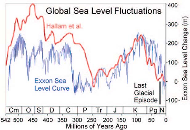 Fig. 9-29. Sea level changes through Earth history. |
Ice Ages of the Pleistocene EpochThe Pleistocene Epoch began about 2.56 million years ago. This Pleistocene ice ages are linked to climate changes cause by many factors resulted in the cyclic expansion of continental glaciers in the polar regions of both hemispheres. Important factors that may have helped initiate the ice ages may be related to plate tectonics.Studies of ice cores from Antarctica, Greenland, cores samples derived from ocean sediments, and studies of glacial deposits found on land indicate that there may have been as many as 20 glaciation periods starting during the late Pliocene through the Pleistocene Epochs (during the last 3 million years). Figure 9-30 shows evidence of glaciation cycles for the last 650,000 years based on studies of greenhouse gases preserved in ice core taken from the Greenland Ice Sheet. The rise and fall in sea level is preserved in sediments deposited in restricted coastal and marine sediments. These sediments are well exposed in many places allowing paleoclimate scientist to evaluate the sedimentary record in many locations (such as at Ft. Funston sea cliffs near San Francisco, CA, Figure 9-31). Some of these cycles were more intense than others, and they impacted regions around the world differently. Each of the glaciation cycles was followed by an interglacial warming period in which the continental glaciers retreated (or melted back). We are currently in one of the interglacial warm periods (although it wouldn't feel like that in Greenland or Antarctica where glaciation is still occurring). Plausible Causes Of the Onset of Continental Glaciation Of the Ice Ages• Prior to the ice ages, the passages between the Arctic Ocean and the Pacific and Atlantic Oceans was more open, allowing unhindered ocean circulation between the regions.• Before about 3 million years ago there was open circulation between the Pacific and Atlantic ocean basins. Plate convergence caused the formation and rise of the Isthmus of Panama, shutting off open tropical ocean circulation between North America and South America. • The plate convergence of the Indian subcontinent with Asia caused the rise of the high and extensive Himalayas and Tibetan Plateau, causing significant defection of the Earth's atmospheric circulation patterns. • The interactions of global plant cover, global cloud cover (and precipitation), polar sea ice, and impacts of massive volcanic eruptions may all have possible influence on glaciation cycles. • Other changes in regional and global atmospheric and oceanographic circulation patterns may have been factors. The rise in CO2 concentrations in the atmosphere over the past century add to the complexity of interpreting the causes of the current rise in global temperatures. The total number, extent, and duration of Pleistocene glaciation cycles is unclear. This is because erosion subsequent glaciation cycles largely destroyed evidence of previous glaciations. In addition, glaciation in one region was not exactly synchronous with other regions. This is illustrated by the fact that the last major glaciation cycle ended about about 11,000 years ago, yet both Antarctica and Greenland are both still experiencing ice-age conditions. Current data suggests that there may have been as many as 20 glaciation cycles in the last 2 million years or so. At least 4 of them were major glaciation cycles that are well preserved in continental glacial sediment deposits exposed in parts of central North America (more cycles are recorded in ocean sediments). |
 Fig. 9-30. Glaciations of the late Pleistocene Epoch 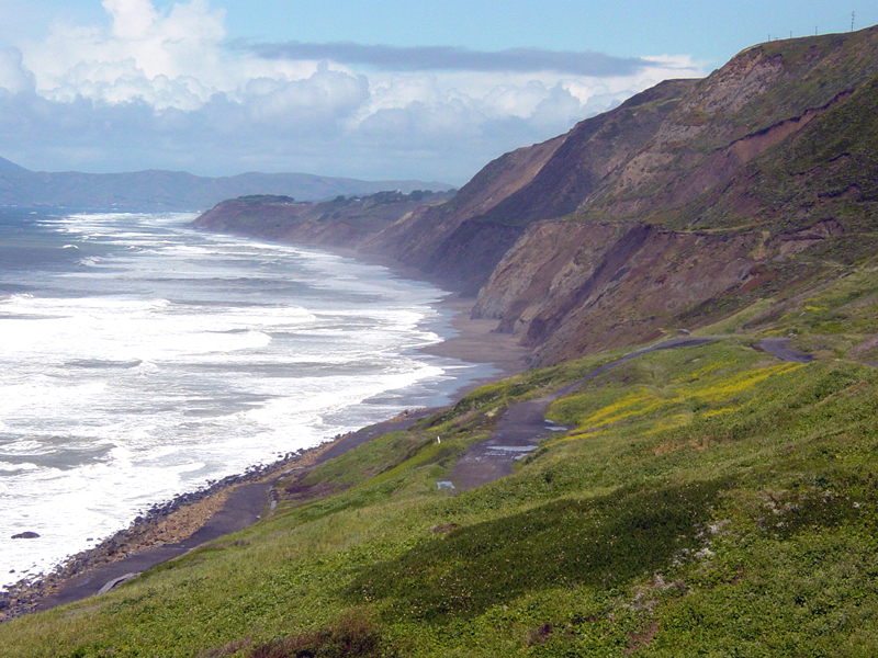 Fig. 9-31. The sedimentary record preserves evidence of numerous glaciation cycles. A famous, well-studied location where a record of sea level changes during the ice ages are well preserved and well in Quaternary-age sediments exposed is in the sea cliffs at Ft. Funston Beach near San Francisco, California. |
Sea Level Changes Caused By Glaciation CyclesThe most recent ice age is called the Wisconsin Stage or Wisconsin Glaciation—it began about 85,000 years ago and ended about 11,000 years ago. The peak of the last ice age, about 26,500 years ago when massive continental ice sheets, ice caps, and alpine glaciers cover much of northern Europe and North America, more extensive glaciers in Antarctica (Figure 9-32). This displaced nearly 10 million cubic miles of ocean water onto the land to be stored as ice. At the peak of the last ice age, glaciers covered about one-third of the land surface. Modern Greenland and Antarctica ice sheet were more extensive than they are today. With water trapped as ice on land, sea level fell around the world by as much as 400 feet below current sea level, exposing all the regions that are now submerged on continental shelves. The location of shelf breaks around the world shows that sea level where coastlines existed at the peak of the last ice age. Research shows that onset of deglaciation began about 20,000 years ago in the Northern Hemisphere with a massive rise in sea level starting starting about 14-15,000 years ago with deglaciation of the West Antarctic Ice Sheet.According to a USGS source, the glaciers currently store about 69% of the world's freshwater (preserved as ice). If all land ice melted the seas would rise about 70 meters (about 230 feet). During the last warm period (an interglacial stade) about 125,000 years ago, sea level rose about 18 feet higher than the current level. About three million years ago, before the major continental glaciation cycle began, sea level was as much as about 165 feet higher than today. |
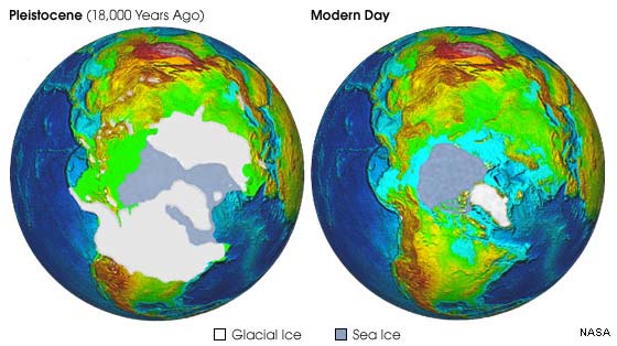 Fig. 9-32. Extent of glaciers and sea ice during the peak of the last ice age and today in the Northern Hemisphere. |
Glacial Cycles Interpreted From Ice Cores and Ocean SedimentsDrilling programs have collected ice cores from the Antarctic and Greenland ice sheets, and many more cores have been collected from marine sediments from around the world. Using geochemical methods and isotopic dating techniques the history of the chemistry of the oceans and atmosphere, and sea level changes through time are well documented (Figure 9-33). For instance, ice has tiny bubbles trapped in them that preserve the chemistry of the air and ice at the time it formed. Sea sediments are loaded with many organic and inorganic materials that can be studied and dated. Shell material of foraminifera contain stable isotopes of carbon and other elements that match the chemistry of seawater at the time that they lived. When glaciers form, the water that forms as ice in polar regions is enriched in light isotopes of oxygen and carbon (light isotopes evaporate from seawater faster than heavy isotopes). As a result, sea water at the peak of glaciation cycles are enriched in the heavy isotopes of carbon and oxygen. The ratios of these isotopes are preserved in microfossil shell material. As a result, scientists have been able to clearly reconstruct a "sea level curve" compared with atmospheric greenhouse gases. |
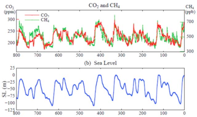 Fig. 9-33. Comparison of concentrations of greenhouse gases with the sea level curve for the last 600,000 years. |
The Astronomical Connection: Milankovitch TheoryEarly in the 20th century, a Serbian geophysicist and astronomer name Milutin Milankovitch worked out mathematically the subtle changes in Earth’s orbital cycles, involving cyclic changes in its rotational axis and its revolution around the Sun changes. Three orbital forcing cycles include the eccentricity of Earth's orbit, Earth's axial precession (41,000 years), precession of equinoxes (21,000 years)(illustrated in Figure 9-34). Eccentricity refers to the change of earth's orbit from being round to more elliptical in shape this cycle repeats every 95,000 years. When it is more elliptical the Earth has shorter, warmer summers and longer, colder winters. Axial precession refers to the wobble in the tilt of Earth's axis. The tilt of the axis changes from about 21.5 to 24.5 degrees on a cycle lasting about 41,000 years. The precession of equinoxes refers to which hemisphere is facing the sun when it is closest to the sun. Right now, the earth is closest to the sun during the winter in the Northern Hemisphere. These cycles impact how much incoming solar radiation that the regions of the earth receive over time, most important being where land is exposed in high latitude regions (where continental glaciation has taken place repeatedly). Milankovitch showed that these cycles combine or interfere with each other in the amount of energy the polar regions receive through time. Climate investigations in the last century have shown that Milankovitch Cycles closely correspond with the record of global temperature changes retrieved from ice cores, marine sediments, and other sources.However, Milankovitch Cycles alone don't explain the onset of the ice ages. |
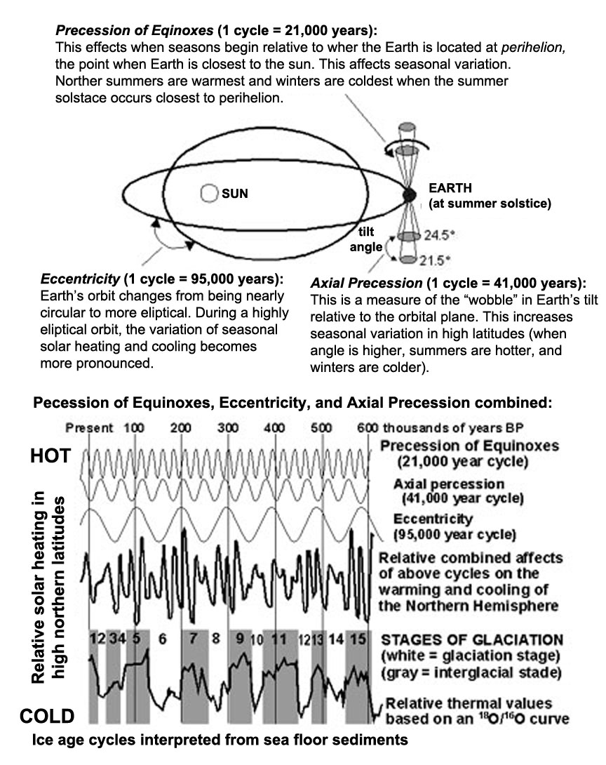 Fig. 9-34. Milankovitch cycles |
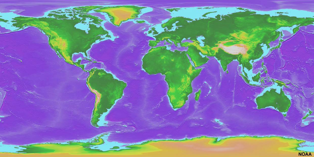
World Oceans and Landmasses During the Ice AgesSea level change since the end of the last glaciation has had major impacts on humans and all "remaining" species alike. A major mass extinction has been on-going since the last ice age. Many will argue that it is because of human over-consumption, but climate change and sea-level-rise have also been major contributing factors (the two factors are linked). When sea level was low, humans (and other species) were able to migrate throughout the world when what are today's continental shelves were coastal plains (Figure 9-35 and 9-36).At the peak of the last ice age sea level about 400 feet (120 m) lower than today. What are now continental shelves were exposed land (coastal plains) that extended out to near the shelf break around continental landmasses. Rivers and streams carved canyons that have flooded as sea level rose, creating fjords, estuaries and bays we see around the world today. Most of the record of human prehistory is now submerged. |
 |
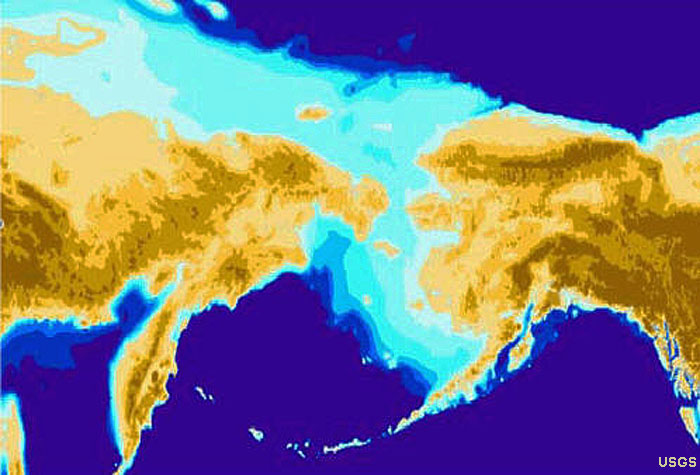 |
| Fig. 9-35. Map of the world with continental shelves shown in light blue. During the peak of the last ice age continental shelves were exposed as extensive coastal plains (allowing humans to migrate). | Fig. 9-36. The continental shelf in the Bering Straits region between Siberia and Alaska was exposed during the last ice age, allowing many species (including humans) to migrate between continents. |
Increasing CO2 Concentrations in the Atmosphere and OceansCO2 concentrations and temperature have tracked closely of the last 300,000 years (Figure 9-37).The recent (if not alarming) increase in CO2 concentrations in the atmosphere is a result of human consumption of fossil fuel, burning forests, and other land use changes. How the Earth's ecosystems are responding to these changes is measurable, and many things are changing. Continental glaciers are melting faster (causing serious concerns about coastal flooding), and the chemistry of ocean water is slowly growing more acidic (endangering ocean species that secrete CaCO3 skeletal material). |
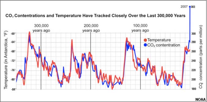 Fig. 9-37. Global temperature and CO2 concentrations over the last 300,000 years. |
Hypoxia and EutrophicationHypoxia is oxygen deficiency in a biotic environment. Eutrophication is caused by excessive amounts of nutrients in a body of water (lake, sea, or parts of an ocean) which causes a dense growth of plant life and death of animal life from lack of oxygen (hypoxia).Excessive amount of nutrients come from runoff from land, with agriculture and sewage being primary contributors. Hypoxia has become a major problem in many parts of the world where whole regions of the seabed are dead or dying because of lack of oxygen. Eutrophication is a serious problem in the northern Gulf of Mexico around the mouth of the Mississippi River delta (Figures 9-38 and 9-39). Seawater density stratification in isolated ocean basins can lead to depletion of oxygen at depth at as microbial decay consumes free oxygen and then starts to break down sulfate ions (-HSO4) to hydrogen sulfide (H2S). Could the Oceans Become Anoxic?Anoxia it the chemical state of bodies of water loosing its free oxygen. This is largely due to density stratification between less dense surface waters and colder, saltier waters at depth. This stratification can cut of upwelling and downwelling, preventing the movement of oxygen into deeper waters.Large portions of the world’s ocean basins have become anoxic in the geologic past. During a million year interval of the Late Cretaceous Period the world’s ocean basins became density stratified. This period is called the Cenomanian-Turonian Oceanic Anoxic Event (OAE). This happened between about 90.5 and 91.5 million years ago (the Cenomanian and Turonian are named epochs of the Cretaceous Period). The world was much warmer in the Cretaceous Period, and there were no continental glaciers. The oceans were warmer, and a thick thermocline and intense pycnocline blocked oxygen-rich surface waters from penetrating deep water. Organic-rich deposits preserved in ocean sediments of the OAE show that there is no bioturbation, suggesting that plankton in the grew in the shallow mixing zone was not consumed if their remains sank into the anoxic condition that existed at the seabed. |
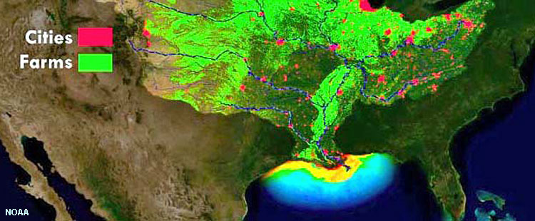 Fig. 9-38. Region impacted by eutrophication in the northern Gulf of Mexico caused by high-nutrient runoff in the Mississippi River system. 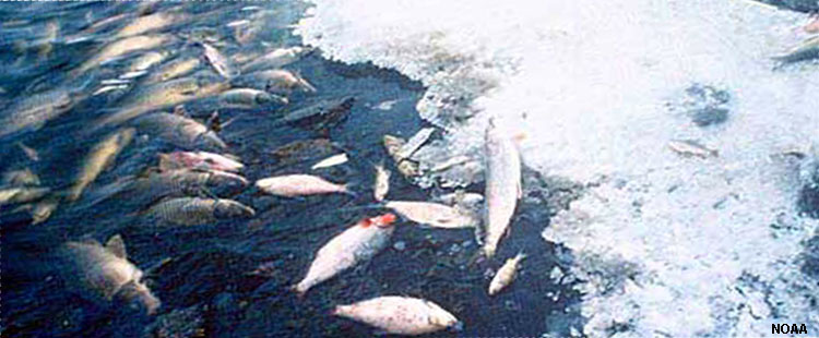 Fig. 9-39. Example of a fish kill caused by hypoxia in a coastal marine environment. Hypoxia increases in the Gulf as water warms up during the summer season. |
Anoxia in the Black Sea BasinDensity stratification can cut of oxygen supply to deep water in restricted basins (including isolated lake basins and inland sea basins). The Black Sea is an example where thermohaline density stratification has lead to anoxic conditions at depth (Figure 9-40). The Black Sea is an inland sea that has anoxic conditions. Marine surface waters flow into the Black Sea from the Mediterranean and Aegean Sea through the shallow Bosphorus Straight (between Greece and Turkey). The Black Sea is a large geographically isolated basin in a semi-arid climate. Normal seawater (less dense) flowing into the basin floats on the surface. With time, high evaporation rates create higher salinity seawater that—with its higher density—sinks in the basin. The denser saline water becomes trapped in the deeper part of the basin is unable to circulate back out of the basin through the shallow Bosphorus Straight. This density stratification produces a strong pycnocline that prevents oxygen in surface waters from reaching depths below about 100 meters. Decaying organic matter that sinks into the deeper, denser seawater consumes all the available oxygen resulting in anoxic conditions below depths of about about about 100 meters. |
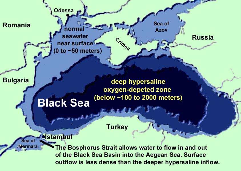 Fig. 9-40. Thermohaline density stratification cuts off oxygen supply to deep water in the Black Sea, causing anoxic conditions below ~100 meters. Normal seawater exists above a halocline in the basin. |
Ocean AcidificationOcean acidification is the reduction in the pH of the ocean over an extended period, typically taking decades or longer. The primarily cause is the uptake of carbon dioxide from the atmosphere into seawater, but can also be caused by other chemical additions or subtractions from the ocean. Examples of ocean acidification are recorded in the geologic record associated with major periods of geologic eruptions and massive extraterrestrial impacts (such as the event that wiped out the dinosaurs along with many groups of marine organisms with shells about 66 million years ago).Anthropogenic ocean acidification refers to the component of pH reduction that is caused by human activity. In the last 250 years, the concentration of CO2 in the atmosphere has increased from 280 parts per million to over 394 parts per million. Most of this is due to the burning of fossil fuels ( coal, gas, and oil) and also by CO2 and other acid-forming compounds released by land use changes (such as burning off forests to be replaced by agriculture). Ocean acidification has potentially devastating ramifications for all forms of ocean life, from microscopic plankton to the largest animals at the top of the food chain. Ocean acidification, increased temperatures, and changing oxygen level are all related, all of which can have catastrophic impacts of marine ecosystems (example in Figure 9-41). |
 Fig. 9-41. Bleaching of coral results death of symbiotic algae living within the corals. This also kills the coral, and is resulting in the collapse of local ecosystems. Elevated water temperatures and acidification are contributing factors. |
What is a Garbage Patch?A garbage patch is a popular name for concentrations of marine debris (mostly small pieces of floating plastic) that accumulate across the more stagnant central parts of the large gyres in the ocean basins. The central regions of ocean basins are areas of convergence and downwelling, so trash from sources on land and sea are carried long distances by currents, much of it ending up in a convergence zone garbage patch. The largest garbage patch is in the north Pacific Ocean (Figure 9-42). Garbage is generally quite hazardous to sea life.(See NOAA's Great Pacific Garbage Patch website.) |
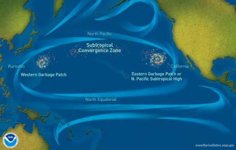 Fig. 9-42. Garbage patches in the Pacific Ocean basin. |
| Chapter 9 quiz questions |