Introduction to Physical Geology

Chapter 6 - Faults, Earthquakes, and Landscapes

6.1

Earthquakes occur somewhere around the world, every hour of every day. Most are too small to even feel—however, large-magnitude, damaging earthquakes happen somewhere around the world almost every year. Large earthquakes in unprepared regions can cause widespread chaos, destruction, and death. Earthquakes are associated with faults, but not all faults currently generate earthquakes (they may have been active long ago). Faults range is size from small fractures in a local outcrop to great fault systems that can extend for thousands of miles.

Fault systems evolve and change over time—driven by plate tectonic forces associated mantle convection influencing the rigid lithosphere. Fault systems are often associated with volcanic regions. Faults may form and remain active for long ages before becoming inactive, and then may become reactivated again in some later period. Tectonic forces within the Earth deform rocks through processes of folding and faulting, producing many of the landscape features observable around us.

This chapter focuses of the examination of faults, their geometry, and how they appear on the natural landscape. It also includes information about earthquakes, earthquake prediction, and earthquake preparedness. Plate tectonics and the internal structure of the Earth are discussed in Chapter 6.

Click on thumbnail images for a larger view.

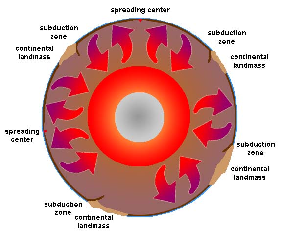Fig. 6-1. Gravitational heat convection in the mantle is the driving force of movement in the Earth's lithosphere.

6.2

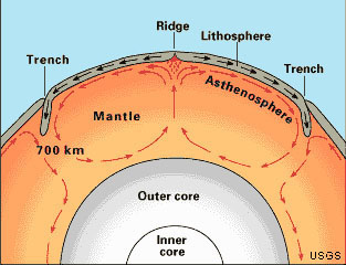
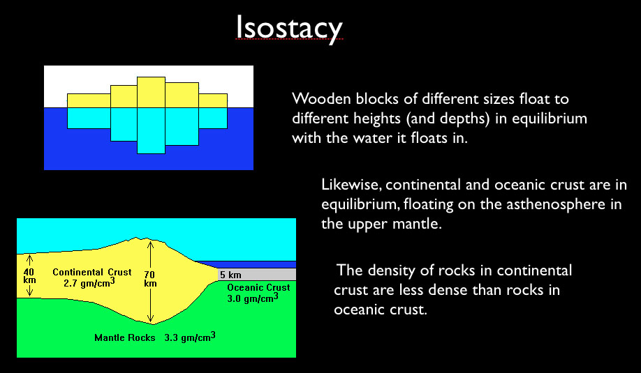
What causes of deformation in the Earth's lithosphere? (An Overview)

Deformation is the action or process of changing in shape or distorting, especially through the application of pressure. In geologic terms, deformation refers to changes in the Earth's lithosphere related to tectonic activity, particularly folding and faulting (discussed below).The term lithosphere is used to describe the Earth's rigid outer layers that include the brittle, rocky crust and underlying upper part of the mantle.

Heat from deep inside the Earth drives gravitational heat convection (hot material expands and rises, cool denser material sinks, Figures 6-1 and 6-2). The rise and fall of masses of material in the mantle create forces that move the rocks in the cool and brittle lithosphere near the Earth's surface. These motions exert great forces, strong enough to rip continents apart, but the rate of movement is generally extremely slow on an annual basis.

Motion within the upper mantle (asthenosphere) is responsible for deep crustal stretching (extension) and compression in the overlying lithosphere. Whereas the fluid-like state of rocks in the asthenosphere move slowly, the solid, brittle material in the lithosphere builds up great pressure (stresses) and the rocks will strain under the pressure until the point that they may rupture rapidly, causing earthquakes that propagates as a shock waves through the Earth.

Isostasy also causes deformation of rocks. Isostatic equilibrium is the state of balance which sections of the Earth's lithosphere (whether continental or oceanic crust) are thought ultimately to achieve when the vertical forces upon them remain unchanged (Figure 6-3). Because continental crust is generally thicker and composed of less-dense grantitic rocks, it floats higher than thinner, denser basaltic ocean crust beneath the world's ocean basins. The lithosphere floats upon the semi-fluid asthenosphere below. For example, If a section of lithosphere is loaded, as by ice, it will slowly subside to a new equilibrium position. During the recent ice ages, great continental glaciers formed on land, causing the crust to sink under the weight of massive ice sheets many miles thick. When the ice melted, the land surface rebounds upward.

Similarly, the crust is always readjusting to changing forces from both above and below. If a section of lithosphere is reduced in mass, as by erosion, it will slowly rise to a new equilibrium position (Figure 6-5). On land, erosion strips away material over time, and isostasy causes the crust to rise. The sediment deposited along continental margins, increases the rock mass, and causes the crust along continental margins to sink.

Fig. 6-2. Gravitational heat convection in the mantle is the source of forces that move, bend, and break rocks in the Earth's lithosphere.

Fig. 6-3. Isostasy: floating wooden blocks of different sizes illustrate how oceanic and continental crustal rocks are at relative isostatic equilibrium floating on the mantle.

Fig. 6-4. Isostatic rebound caused by the melting of continental glaciers reveals the fluid-like behavior of the asthenosphere. Isostasy can create immense pressure that can cause earthquakes.

Fig. 6-5. Isostatic adjustments occur as erosion strips away rocks as mountainous landscapes erode away, removing sometimes miles of rock over time.

6.3

Igneous Activity Can Cause Crustal Deformation

Heat rising from the mantle can cause rocks to expand, causing them to loose density and rise. In addition molten material derived from the lower crust and mantle is typically under great pressure, and can force its way through fractures and zones of weakness. Migrating magma displaces and deforms rocks as the molten material forces its way upward, often filling balloon-like magma chambers deep in the subsurface. It will also displace or deform rocks while forcing its way toward the surface to create volcanoes. Massive volcanic eruptions are associated with faulting and commonly occur in association with intense earthquake activity. Massive asteroid impacts that occurred throughout Earth history have also caused massive local and regional deformation, shattering and melting rocks from shock waves associated caused by their impact.

6.4

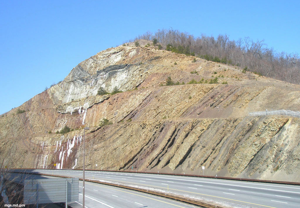
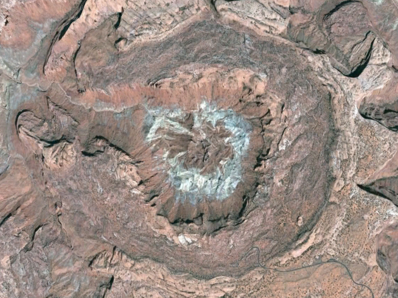
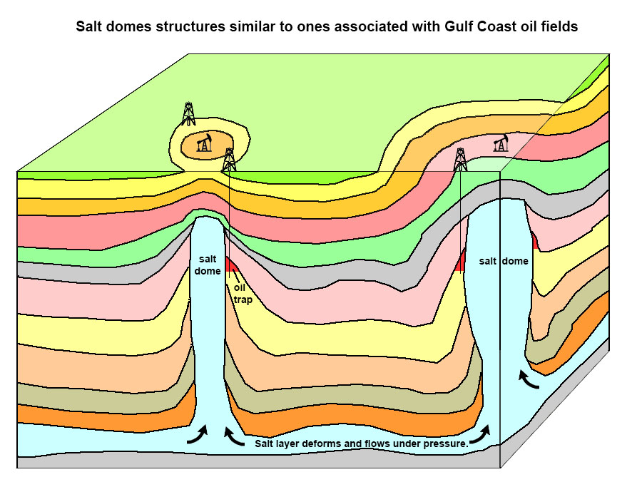
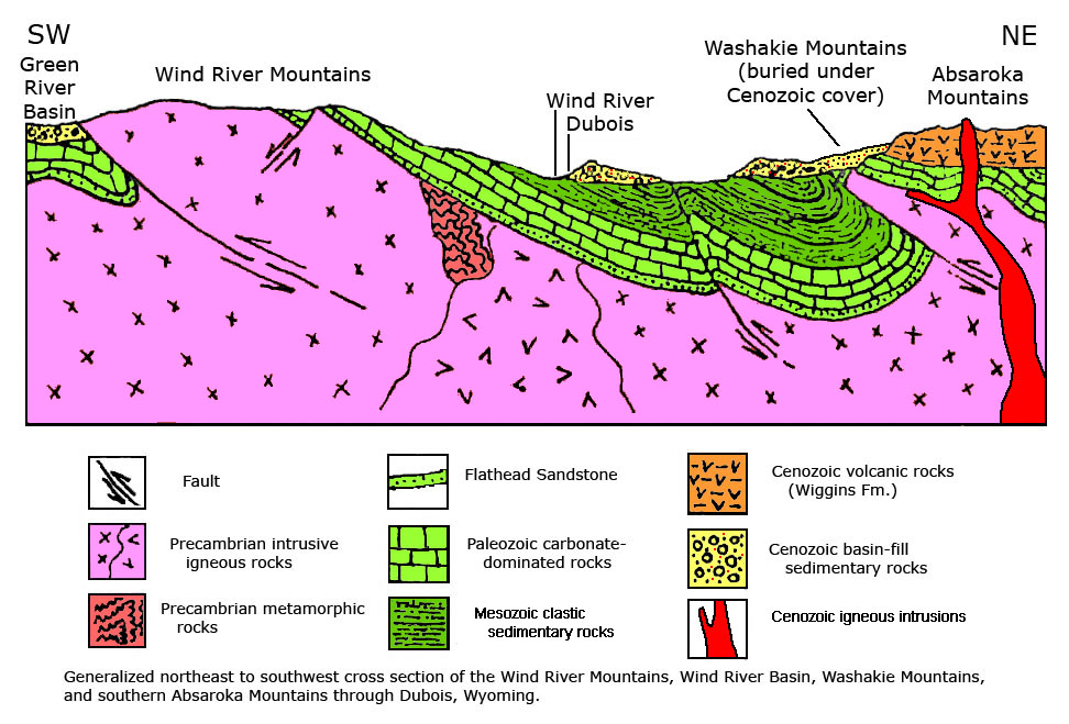
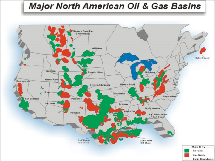
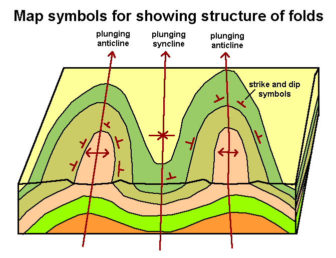
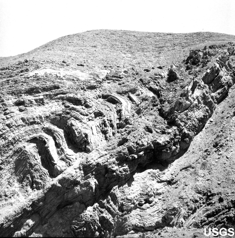
Types of Folds

All kinds of rocks are subject to deformation forces, but the effects are most easy to observe in stratified rocks that originally accumulated as flat layers (sedimentary layers or volcanic lava flows and ash deposits). A geological fold occurs when one layer or a stack of originally flat and planar surfaces are bent or curved as a result of permanent deformation. Folding is the bending or warping of stratified rocks by tectonic forces (movements in the Earth's crust). Folds can be observed on many scales, for tiny folds as can be seen in hand specimens, to larger scales as can be seen on the sides of road cuts or canyons, or very large scale such as entire mountain ranges to features that are so large they can only be seen from airplanes or satellites. Folds typically have a linear orientation that has a defined axis, similar to the orientation of the crest of a roof line or a trough of a gutter.

Figure 6-6 illustrates different types of folds.

An anticline is a fold in layers of rock (strata) where the concave side faces down, with strata sloping downward on both sides from a common crest [axis] (Figure 6-6).

A syncline is a trough-shaped fold of stratified rock in which the strata slope upward from the axis; opposite of an anticline (Figure 6-7).

Plunging folds are folds (anticlines or synclines) that are tipped by tectonic forces and have a hinge line not horizontal in the axial plane (Figures 6-9 to 6-10).

A dome is a deformational feature consisting of symmetrically-dipping anticlines; their general outline on a geologic map is circular or oval (Figures 6-11 to 6-12).

A basin is s structural downwarp, a doubly plunging syncline ,or more typically, a downwarp filled with sediments derived from surrounding areas. The term basin is used to describe a large-scale structural formation of rock strata formed by tectonic down warping of previously flat lying strata. Structural basins are geological depressions, and are the inverse of domes. Some elongated structural basins are basically large synclines. Some structural basins are exceedingly large and are host to major oil and gas reservoirs and coal fields in the United States (and around the world) (Figures 5-13 and 6-14).

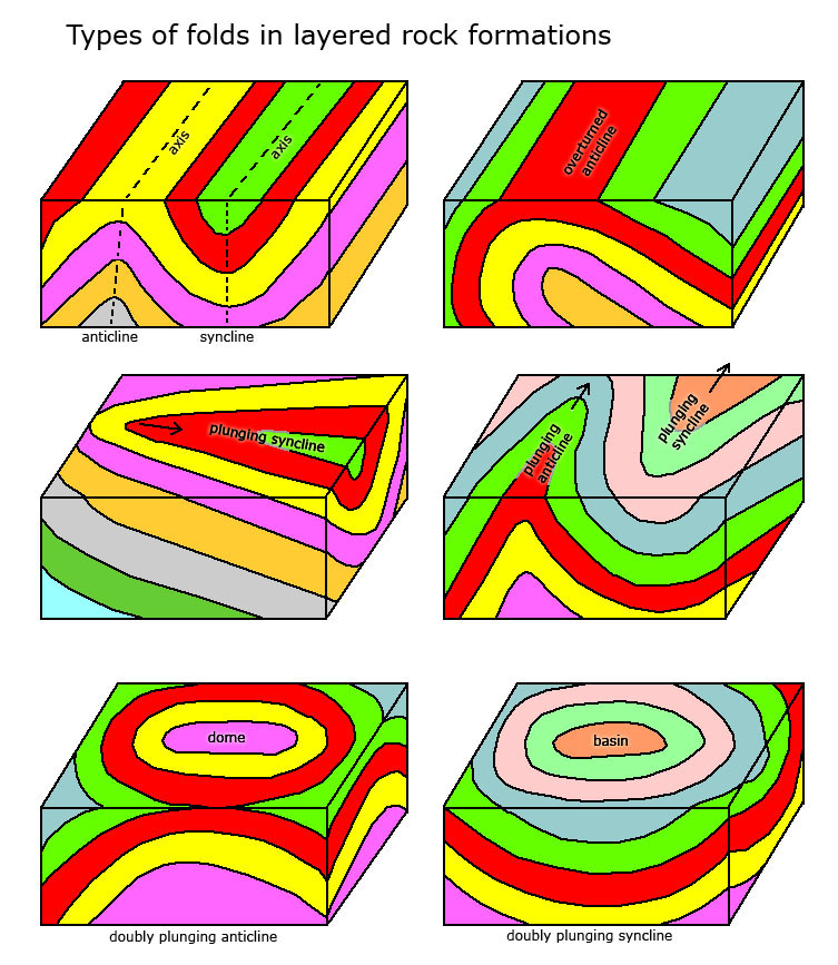Fig. 6-6. Folds illustrated with block diagrams: anticline, syncline, an overturned fold, a plunging syncline, plunging anticline and syncline, a dome, and a basin.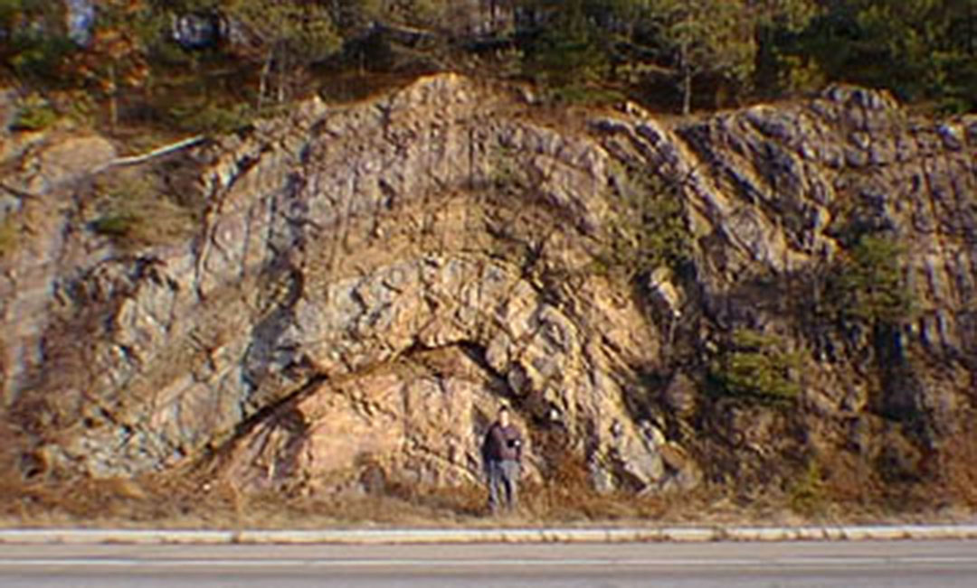

Fig. 6-6. An anticline and syncline exposed in a road cut along Route 23 near the town of Butler in northern New Jersey. Strata displaying anticlinal fold arch up in the middle; a syncline forms a smile-like trough.

Fig. 6-6. A syncline exposed along a cut through Sideling Ridge along Interstate 68 in western Maryland. This fold is a cross section of similar ridges in the Appalachian Mountains as shown in Figure 6-10.

Fig. 6-8. Plunging syncline
exposed by low tide at the Fitzgerald Marine Preserve
in San Mateo County near San Francisco, California. Plunging synclines have an axis that dips in one direction.

Fig. 6-9. Plunging folds as viewed from a satellite image of a portion of the Bighorn Basin, Wyoming. It is not uncommon for anticlines and synclines, whether plunging or not, to occur adjacent to one-another.

Fig. 6-10. Forested ridge lines of sedimentary rock stand out as plunging folds (anticlines and synclines) in this view of part of the Valley and Ridge Province in the Appalachian Mountains near Harrisburg, Pennsylvania.

Fig. 6-11. Upheaval Dome, a circular dome in Utah's
Canyonlands National Park is an dearly circular dome.

Fig. 6-12. Block diagram illustrating salt domes associated with some oil fields in the Texas-Louisiana Gulf Coast and offshore regions.

Fig. 6-13. This cross section of Wind River Basin in Wyoming showing the great synclinal fold structure of strata of the basin.

Fig. 6-14. Map of large geologic basins in the United States where locations of oil and gas deposits occur.

6.5

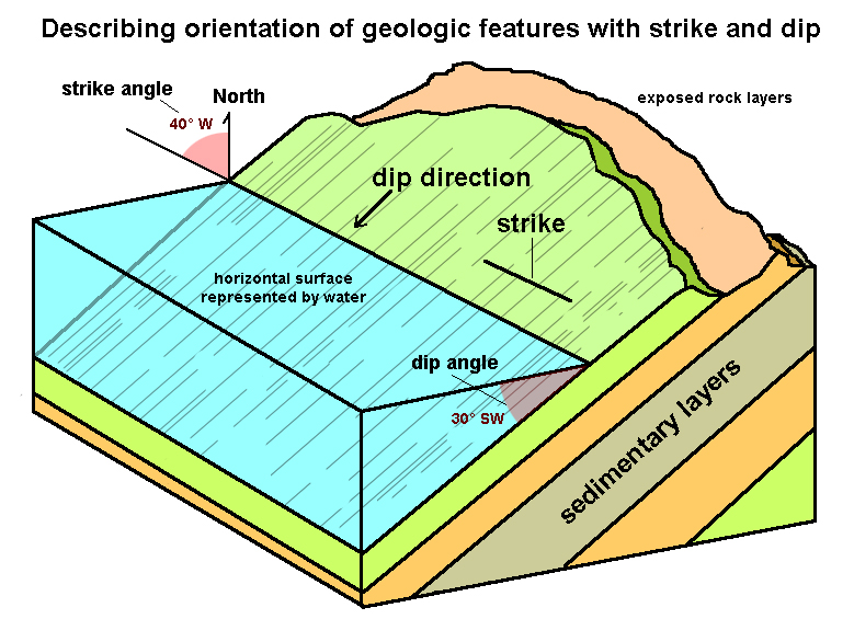
How are structural features described and illustrated on maps and cross sections?

Geologists use the terms strike and dip to describe the orientation of layers of stratified rocks exposed at the earth surface ( 6-15). Strike and dip are well illustrated by the Strike Valley in Capitol Reef National Park in Utah (Figure 6-16).

Strike is the direction taken by a structural surface, such as a layer of rock or a fault plane, as it intersects the horizontal. Strike is measured in degrees east or west of true north.

Dip is the angle that a rock layer or any planar feature makes with the horizontal, measured perpendicular to the strike and in a vertical plane. Dip angles can range from 0 (zero) degrees for horizontal beds, to 90° for vertically inclined beds, or higher numbers up to 180° for beds that are completely overturned.

Describing strike and dip: The strike and dip of a bed might be written with strike designation before dip. Examples: N35°W, 15°W or N22°E, 18° E. Note that the dip direction is contingent on strike, and the W or E for the dip direction only describe if the beds are incline downward in a westerly or easterly direction. Note, if the beds are horizontal, there is no strike and dip designation!

Strike and dip measurement are illustrated on geologic maps using lines, arrows, and special T-shaped dip symbols (Figures 6-17).

Figure 6-18 uses block diagrams to illustrated common map symbols used on geologic maps including different kinds of folds and faults.

Fig. 6-15. Describing orientation and inclination of rock strata and geologic features with strike and dip.

Fig. 6-16. A view illustrating strike and dip from the Strike Valley Overlook in Capitol Reef National Park, central Utah.

Fig. 6-16. Illustrating symbols for plunging folds on geologic maps. Arrows and dip symbol show the orientation of strata.

Fig. 6-18. Common map symbols used on geologic maps including different kinds of folds and faults.

6.6

Rocks Shattered and Broken By Tectonic Forces

Joints - Fractures In Rocks

Many types of rocks are very brittle and will shatter (like glass) if subjected to pressure or a shock wave from an earthquake, producing fractures. Old rocks exposed in mountainous regions typically appear shattered with fractures running in many directions. Sometimes there is a dominant fracture direction or orientation pattern.

A simple crack in a rock that displays no apparent offset is called a joint. A joint is a fracture in rock where the displacement associated with the opening of the fracture is greater than the displacement due to movement in the plane of the fracture (up, down or sideways) of one side relative to the other. If a fracture does not have obvious offset it is a joint. If a fracture displays offset it is a fault (Figures 6-19 and 6-20 show examples of joints).

Fig. 6-19. Joints in sandstone
Checkerboard Mesa
Zion National Park, Utah

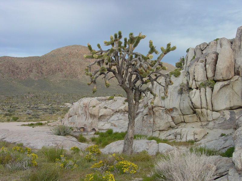Fig. 6-20. Joints in granite
Joshua Tree National Park, California

6.7

Features Associated With Faults

A fault is a fracture or crack along which two blocks of rock slide past one another. This movement may occur rapidly, in the form of an earthquake, or slowly, in the form of creep (Figure 6-20). Types of faults include strike-slip faults, normal faults, reverse faults, thrust faults, and oblique-slip faults. Faults can be small to large complex systems of interlinking faults and may change form one kind of fault in one location to another kind somewhere else. Many faults are associated with folds. Faults split, bifurcate, merge, or can peter out over distances, sometime forming complex systems of fractures.

The relative motion of faults (one side to the other) is described in terms of relationship of a hanging wall and foot wall (see normal fault and reverse fault examples in Figure 6-20).

A foot wall is the underlying block of a fault having an inclined fault plane.

A hanging wall is the block (rocks) on the upper side of an inclined fault plane.

Simply described here—if a fault is exposed well enough to see that the fault plane is inclined, the side you could stand on is called the foot wall. The side you could hang from without your feet touching the ground is the hanging wall.

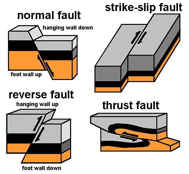Fig. 6-20. Block diagrams illustrating common types of faults: normal fault, reverse fault, strike-slip fault, and thrust fault. Offset strata illustrates the relative motion of the foot wall to the hanging wall of each type of fault.

6.8

Types of Faults

There are three types of dip-slip faults: normal, reverse, and thrust (Figure 6-21). The character of the movement (offset) along the fracture plane determines what kind of dip-slip fault it is.

If the rock mass above an inclined fault moves down, the fault is termed normal, whereas if the rock above the fault moves up, the fault is termed reverse. A reverse fault in which the fault plane is inclined at an angle equal to or less than 45° is called a thrust fault.

A normal fault is a fault in which the hanging wall appears to have moved downward relative to the foot wall. The dip angle of the slip surface is between 45 and 90 degrees. Many normal faults in mountainous regions form from gravitational pull along mountainsides and may be associated with the headwall escarpment of slumps (examples: Figures 6-22 and 6-23).

A reverse fault is a fault in which the hanging wall has moved up relative to the foot wall (example: Figure 6-24).

A thrust fault is a fault with a dip angle of 45º or less over its extent on which the hanging wall appears to have moved upward relative to the foot wall (example: Figure 6-25). Horizontal compression or rotational shear is responsible for displacement. (See also reverse fault and oblique-slip fault.)

A strike-slip fault is a generally vertical fault along which the two sides move horizontally past each other (examples: Figures 6-26 and 6-27). If the block opposite an observer looking across the fault moves to the right, the slip style is termed “right lateral.” If the block moves to the left, the motion is termed “left lateral.” California’s San Andreas Fault is the most famous example of a right-lateral strike-slip fault. Strike-slip faults produce produce a variety of landforms including shutter ridges, pull-apart basins, sag ponds, and deflected streams.

Oblique-slip faults are faults that display significant components of both horizontal (strike-slip) and vertical (dip-slip) motion. An oblique-slip fault combines strike-slip motion with significant normal, reverse, or thrust offset.

Fig. 6-22. Normal fault: Anza Borego State Park, San Diego County, CA.	Fig. 6-23. Normal fault: Gazos Creek State Beach, CA	Fig. 6-24. Reverse fault along the mountain range front, Arroyo Seco Canyon, CA
Fig. 6-25. Thrust fault: Atacama Province, Chile	Fig. 6-26. Strike-slip fault: aerial view of the San Andreas Fault exposed in Carrizo Plain National Monument, CA	Fig. 6-26. Fence line offset by right-lateral strike-slip movement on the San Andreas Fault near San Juan Bautista, CA

6.9

Descriptions of Fault Characteristics

Geologists will first describe the kind of fault (normal, reverse, thrust, strike-slip, etc. see Figure 6-20). Strike and dip is also used to describe the orientation of fault surfaces and use special symbols to describe them on a map (see Figure 6-18). Small arrows are commonly used to indicate relative offset motion along a fault on an illustration or map. Geologist also use selected terms to describe faults as they appear on the land surface:

A fault line is the intersection of a well-defined fault plane with the land surface. A fault is typically illustrated as a line on a map.

A fault zone is an area of many closely spaced faults and fractures that collectively can be mapped within a continuous zone. There may be more than one fault line in a fault zone! (Figure 6-28).

A fault system is a collection of many faults and are complex. A fault system may have a variety of faults and fold structures that may bifurcate and merge, change orientation, may be discontinuous, terminate, or peter out gradually. A fault system is a collection of parallel or interconnected faults that display a related pattern of relative offset and activity across an entire region (for example, the California Fault System includes the San Andreas Fault and many associated faults throughout the region; Figure 6-29).

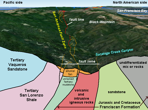Fig. 6-28. Fault line and fault zone illustrated for the San Andreas Fault in the Santa Cruz Mountains near San Jose, California. The San Andreas Fault is part of the greater California Fault System which consists of numerous parallel and intersecting faults across the region.

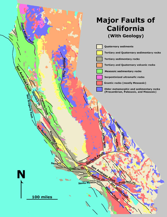Fig. 6-29. The California Fault System shown on a generalized geologic map in California

6.10

Stress and Strain

The terms stress and strain are terms commonly used in mechanical engineering, but are also practical terms for describing the behavior of earth materials subjected to tectonic forces.

Stress is the force acting on a rock or another solid to deform it, measured in kilograms per square centimeter or pounds per square inch.

Strain is the amount of deformation an object experiences compared to its original size and shape.

Rocks, like any solid material, when subjected to a stress will respond with a strain. However, the character of the strain depends on the material strength of the rock. For instance, a hard rock like granite make take on a large amount of stress without showing any significant deformation, but at at some point with increasing pressure it will shatter (fracture) catastrophically. On the other hand, shale, a very soft rock, will deform (fold) significantly before it ruptures as a fault.

Crustal Compression vs. Crustal Tension

On a regional scale, rocks are subjected to stress that may be compressional (such as along a convergent plate boundary) or tensional (such as along a rift valley or a spreading center of a divergent plate boundary). The faults in the vicinity of these stress forces produce faults and features that can be described as crustal shortening or crustal extension (Figure 6-30). Crustal compression is more likely to form thrust faults and reverse faults associated with crustal shortening, and crustal compression is typically associated with regions where mountain ranges are being pushed up. In contrast, crustal tension is more likely to form normal faults associated with crustal extension. Continental rifting and associated crustal thinning are associated with crustal extension.

Shearing stress is a force that occurs where opposing sides of a zone within the crust move in opposite directions, resulting in rotational bending and/or the formation of strike-slip faults or oblique slip faults. Shearing stress can result in formation of complex fault systems with many moving parts resulting in a variety of fault and fold patterns and associated landscape features (discussed below).

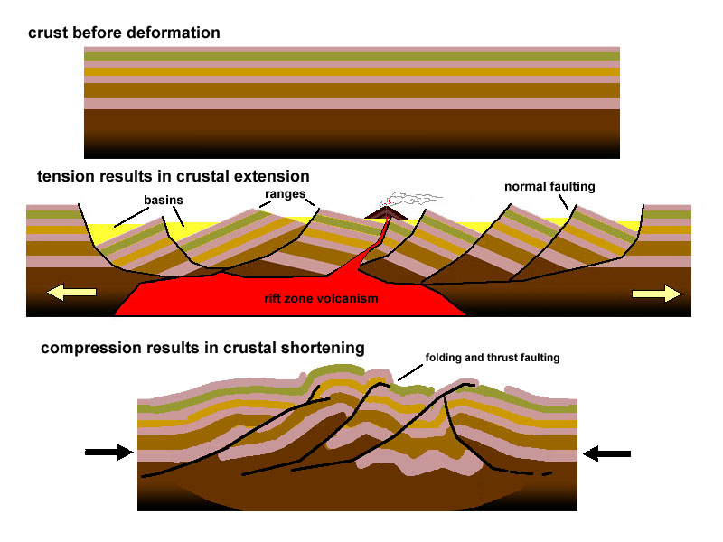Fig. 6-30. Compression results in crustal shortening whereas tension results in crustal extension. Crustal shortening typically results in thrust faults or reverse faults. Crustal extension produces mostly normal faults.

6.11

Brittle vs. Ductile Deformation

Rocks near the surface are cold, but the temperature deep down can be extremely hot. Cool rocks near the surface tend to shatter (forming joints and faults) when they rupture. Deep underground, the weight of overlying material adds confining pressure to hold rocks together, and if hot enough they will deform fluidly rather that fracture if heat and pressure is great enough.

Rocks under high confining pressures and temperatures at depth will bend (fold) and stretch, whereas cool and brittle rocks closer to the surface will break (fracture) under increasing pressure. An imaginary plane exists in the lower crust and upper mantle above which rocks will tend to break (causing earthquakes) but below which they will tend to deform like plastic under pressure. This hypothetical boundary is called the brittle-ductile transition zone (Figure 6-31). This zone varies significantly with depth and subsurface temperatures from one region of the lithosphere to another, often reflecting plate boundary conditions.

The deepest (and strongest) earthquakes typically occur where cold oceanic crust sinks deep into the asthenosphere along subduction zones. Cold ocean crust remains brittle as it sinks along a subduction zone. A great amount of pressure builds up on the sinking slab, and where it is still cold and brittle enough to fracture, producing powerful earthquakes. Deeper in subduction zones, the sinking rock heats up and will bend or flow under the greater pressure rather than fracture.

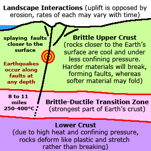Fig. 6-31. The upper crust behaves in a brittle fashion, fracturing under strain (producing earthquakes), whereas at depth rocks deform plastically, folding or flowing under pressure rather than fracturing (no earthquakes).

6.12

Phenomena Associated With Earthquakes and Earthquake Faults

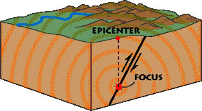Fig. 6-32. Diagram illustrating the epicenter and focus of an earthquake along a fault.

Terms used to describe earthquakes (illustrated in Figure 6-32):

An earthquake is ground shaking caused by a sudden movement on a fault or by volcanic disturbance.

An epicenter is the point on the Earth’s surface above the point at depth in the Earth’s crust where an earthquake begins.

The focus is the point below the Earth's surface where seismic waves originate during an earthquake.

6.13

Faults and Earthquake Faults

An earthquake fault is an active fault that has a history of producing earthquakes or is considered to have a potential of producing damaging earthquakes on the basis of observable evidence. Not all faults are active or are considered earthquake faults. However, faults can remain dormant for long periods of time and can be reactivated by changing stress patterns in the crust. Below are key terms used to describe earthquake phenomena.

An earthquake is the sudden and sometimes violent shaking of the ground as a result of movements within the crust associated with fault rupture or volcanic activity. Earthquakes are described in terms of magnitude and intensity (discussed below). Earthquakes can also be a result of a landslide or an explosion (such as a mining or demolition blast, bomb testing, or potentially an asteroid impact, or anything that creates a shockwave).

Fault creep is the gradual movement (displacement) displayed by a fault over time. Fault creep generally keeps pace with regional plate-tectonic related movement in a area. Creep is the aseismic movement of a fault (movement without detectable earthquakes). Active earthquake faults can produce both earthquakes and creep. (Note that the word creep is also used for the slow movement of soil down a slope.)

A rupture zone is the area through which fault movement occurred during an earthquake. For large earthquakes, the section of the fault that ruptured may be several hundred miles in length. Note that ruptures associated with earthquakes may or may not extend to the ground surface. In addition, shockwaves produced by one earthquake fault, may also set off earthquakes on other faults.

6.14

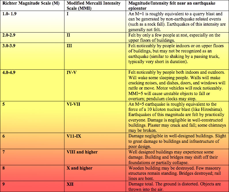
Seismic Waves

Seismic waves are shock waves and vibrations in the Earth which issue from the focus of an earthquake—it may be a result of an earthquake, impact, or explosion, or some other process that imparts low-frequency acoustic energy (Figure 6-33).

A P wave (P) is a compressional wave is a seismic body wave that shakes the ground back and forth in the same direction and the opposite direction as the direction the wave is moving. A P wave is the first shock wave to arrive from an earthquake at a distant location.

A S wave (S) is a shear wave is a seismic body wave that shakes the ground back and forth perpendicular to the direction the wave is moving.

A seismograph is a device used to record earthquake shaking and are used to determine the distance, magnitude and intensity of earthquakes. Data from numerous seismographs linked together in networks are used to determine the focus, epicenter, extent of rupture, and amount of shaking in a region caused by an earthquake. A minimum of 3 seismographs are needed to determine the epicenter of an earthquake (Figure 6-34). Today there are many thousands of seismographs connected to networks that can record earthquake information from around the world.

A person who studies earthquakes and earthquakes faults is called a seismologist.

Speed of P waves and S waves are used to determine the location of an earthquake

P waves (primary compression shock waves) move about 4 miles per second (5 to 8 km/second) depending on the density and character of crustal rocks. (The actual range is between 3 to 5 miles per second or 5 to 8 km/second).

S waves (secondary shear or shake waves) move about 60% as fast as P waves in the same crustal rocks.

Because compression (P) waves travel faster than shear (S) waves: Using a precision clock and three seismographs, the location of an earthquake epicenter can be precisely located by measuring the arrival times of the first P wave and the first S wave (illustrated in Figure 6-34).

Example: Suppose you feel an earthquake's P and S waves arrive 5 second apart. Assuming P waves moving at 5 miles per second and S waves moving 3 miles per second (60% of the P wave), the epicenter of the earthquake was 10 miles away [calculation: (5 mi/sec - 3 mi/sec) x 5 sec = 10 miles].

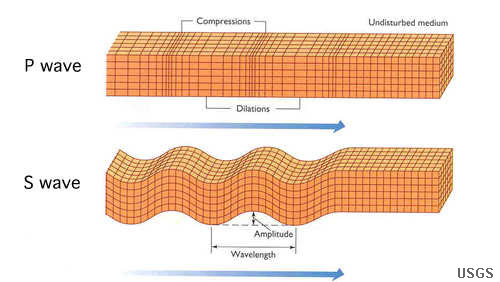Fig. 6-33. Earthquake waves include:
P waves (compression wave) and S waves (shear waves0
P-waves move faster than S-waves and are first to be felt, the S-waves arrive next and produce the majority of shaking in an earthquake.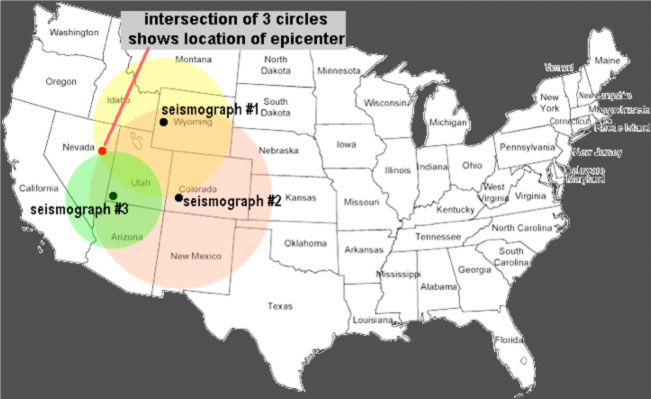

Three seismographs locating the epicenter of an earthquake

Fig. 6-34. At least three seismographs are needed to locate the epicenter of an earthquake. A single seismograph can only tell you how far away an earthquake occurred, but not in which direction (a circle). Where three seismograph circles intersect is the location of an epicenter.

6.15

Earthquake Foreshocks, Aftershocks, and Main Events

Earthquakes can be complex events. An earthquake may be described as a single shock wave or a complex pattern of shock waves taking place over a period of time. Typically in large earthquakes, there is a main event associated with the largest shock wave and significant rupture, but there there may be a series of foreshocks and aftershocks created as the fault rupture propagates through the crust, releasing or dispersing energy. It is similar to when a rock hits a windshield on a car. the initial bang causes the event, but the cracks propagate across the window, releasing the pressure in the glass as it shatters. Sometime small earthquakes happen before a main earthquake event—these are called foreshocks. More typically, there are often numerous smaller magnitude earthquakes after a main shock event—these are called aftershocks. Unfortunately, it is impossible to truly define a foreshock before a larger-scale earthquake. Both foreshocks and aftershocks can take place from seconds, minutes, hours, days, weeks, years, and even longer periods associated with a main earthquake event.

Can we tell if an earthquake is a foreshock to a larger impending earthquake? The answer is a definite "maybe." Some earthquakes do not have foreshocks. The seismic history of the major faults in some regions are well known. Faults, like the San Andreas Fault, are defined as segments based on earthquake history, bedrock geology, and associations with intersecting faults (Figure 6-35). For instance, some segments of the San Andreas Fault have experienced major earthquakes, releasing pent-up pressure on a segment or segments of the fault. Some segments of the fault are creeping and are not likely to produce great earthquakes as in other segments (in theory). Still other segments of the fault are locked up and have not experienced a major earthquake in historic times. It is these locked up segments that are of significant concern, and any small earthquake or series of small earthquakes in the vicinity of these segments are considered possible foreshocks to a possibly larger main shock and possible aftershocks to follow.

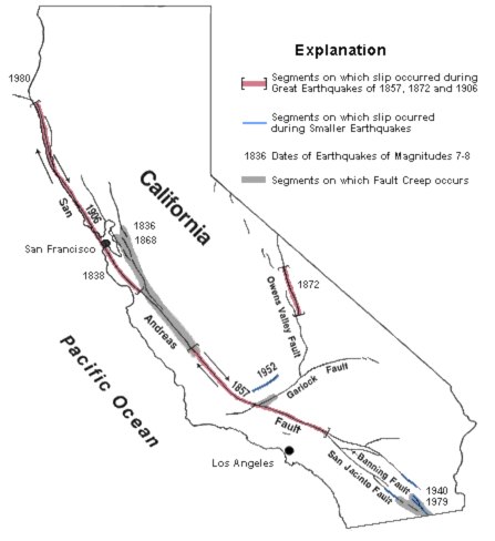Fig. 6-35. The San Andreas Fault and other faults in the California Fault System are subdivided into many segments based on seismic history, local geology, and intersections with other faults.

6.16

Earthquake Magnitude and Earthquake Intensity

The energy released by earthquakes are measured or described in two ways: earthquake magnitude and earthquake intensity (Figure 6-36).

Earthquake magnitude (M) is a numeric measure that represents the size or strength of an earthquake, as determined from seismographic observations. The Richter scale is a numerical (logarithmic) scale for expressing the magnitude of an earthquake on the basis of seismograph oscillations data. Today earthquake intensity is recorded with a moment magnitude scale (MMS) which is based on the seismic moment of the earthquake, which is equal to the rigidity of the Earth multiplied by the average amount of slip on the fault and the size of the area that slipped. Richter scale and moment magnitude scales are similar, but the MMS scale is more precise.

Earthquake intensity (I) is a measure of ground shaking describing the local severity of an earthquake in terms of its effects on the Earth’s surface and on humans and their structures. The Modified Mercalli Intensity (MMI) scale, which uses Roman numerals, is one way scientists describe earthquake intensity (see Figure 6-36).

Fig. 6-36. Comparison of earthquake magnitude (MMS) and intensity (MMI) scales (USGS).

6.17

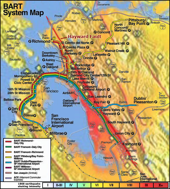
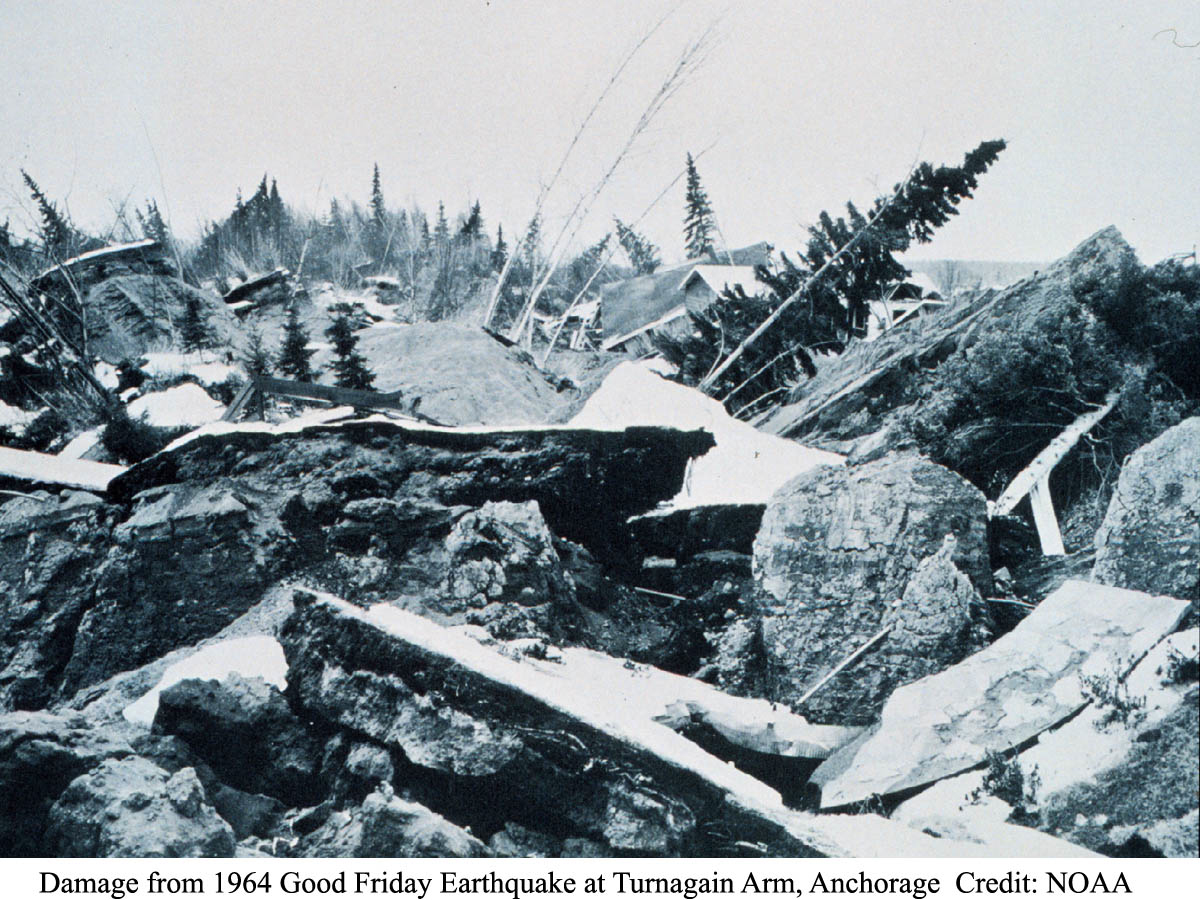
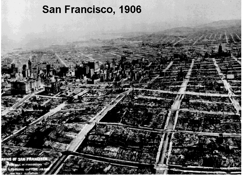
Naming of Significant Earthquakes

Large, damaging earthquakes are typically named for a well-known named location or region near or around the epicenter of an earthquake and the year that it occurred. For example, the Great San Francisco Earthquake of 1906 or the Great Midwest Earthquake of 1811. The addition of the word great to a name implies great destruction was associated with an historically massive earthquake (which, really, isn't all that great!). Typically the maximum magnitude of the earthquake is also reported with earthquakes if the maximum magnitude was accurately/precisely determined, such as the M9.2 Great Alaska Earthquake of 1964. Interestingly, the name Great San Francisco Earthquake was applied to the 1868 earthquake on the Hayward Fault, but the name was switched to the even greater 1906 earthquake on the San Andreas Fault. Neither fault runs through San Francisco, but that is where the destruction occurred.

6.18

Seismic Networks

The US Geological Survey manages a national seismic network to collect earthquake data. This network is a collaboration with many organizations and universities involved in seismic research.

The USGS maintains part of the Global Seismographic Network which consists of thousands of seismographs around the world, so information about earthquakes can be calculated quite precisely. Below are examples of earthquake fault maps and earthquake hazard assessment maps of portions of the United States.

6.19

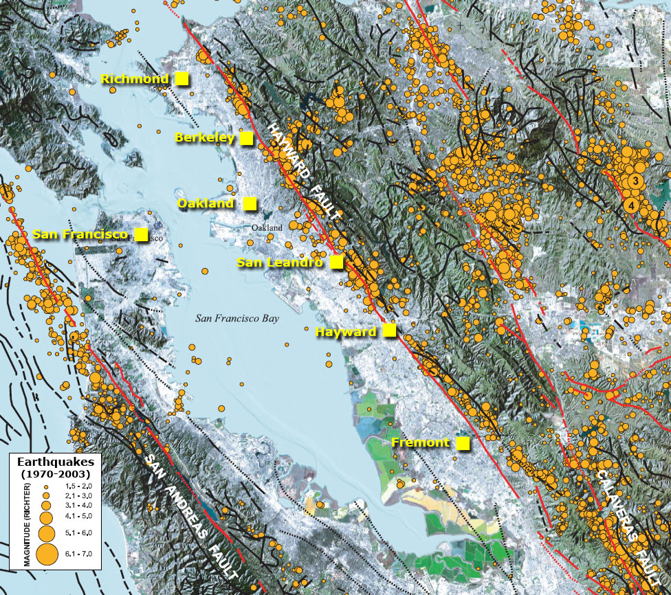
Selected Maps Illustrating Fault and Earthquake Data

Figure 6-37 is a map of faults in the San Francisco Bay region showing the location epicenters of historic earthquakes of varying intensity. Note that epicenters are not always on mapped fault lines because the focus of earthquakes occur on faults below the surfaces.
Figure 6-38 is a map showing the predicted intensity of a strong earthquake if one were to occur (as it has in the past) on the Hayward Fault.
Figure 6-39 is a map showing strong earthquake hazard regions of the United States. The map shows that the active margin of North America's West Coast is a region with a long history of powerful earthquakes. The red area in the Mississippi River Valley region is associated with the New Madrid (Missouri) Fault Zone which produced two of the strongest earthquakes in US history (in 1811 and 1812). The red area on the East Coast is associated with the Great Charleston Earthquake of 1886.

Check out these map posters for earthquakes and faults in southern and northern California!

Sleeter, B.M., Calzia, J.P., and Walter, S.R., 2012, Earthquakes and faults in southern California (1970–2010): U.S. Geological Survey Scientific Investigations Map 3222, scale 1:450,000. (Available at https://pubs.usgs.gov/sim/3222/.)

Sleeter, B.M., Calzia, J.P., and Walter, S.R., Wong, F. L. and Sausedo, G.J., 2004, Earthquakes and faults in the San Francisco Bay Area (1970-2003): U.S. Geological Survey Scientific Investigations Map 2848, scale 1:450,000. (Available at https://pubs.usgs.gov/sim/2848/.)

Fig. 6-36. Earthquake fault lines and epicenters map of the San Francisco Bay region (USGS). Note that earthquake epicenters don't line up with fault lines on the surface.

Fig. 6-38. Predicted earthquake intensity map of the Hayward Fault, California (USGS).

Fig. 6-39. Earthquake hazard map of the United States (USGS) - areas of greatest risk are shown in red and are based on historic earthquake information and seismic studies of known earthquake faults.

6.20

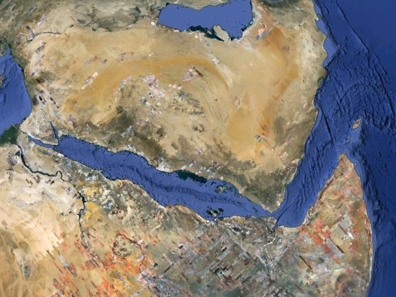
Landscape Features Associated With Faults

There are a wide variety of landscape features (small to very large) associated with faults. Fault movements and weathering and erosion processes combine to create a variety of landscape feature. It the long run, erosion tends to dominate and destroy or cover evidence of activity associated with fault motion, but often the location of faults can be recognized by patterns on the landscape. Examples are described below:

A graben is an elongate, structurally depressed crustal area or block of crust that is bounded by faults on its long sides. A graben may be geomorphically expressed as a rift valley or pull-apart basin. Grabens are commonly associated with horsts (Figures 6-40 and 6-41).

A horst is a raised elongated block of the earth's crust lying (or rising) between two faults.

A rift valley is a valley that has formed along a tectonic rift. Rift valleys may be grabens or pull-apart basins, may be structurally complex, and are typically modified by erosion. The Red Sea is a flooded rift valley (similar to the African Rift valleys)(Figures 6-42 and 6-43). Rift valleys form as a result of crustal extension and may become divergent plate boundaries.

Fig. 6-40. Horsts and grabens form from crustal extension.

Fig. 6-41. Horsts and grabens
Canyonlands National Park, Utah (Google satellite image)

Fig. 6-42. Red Sea rift area (USGS data and Google satellite image)

Fig. 6-43. Map showing the location of the African Rift Valleys

6.21

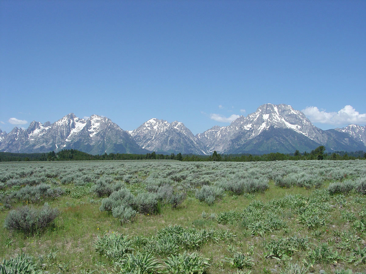
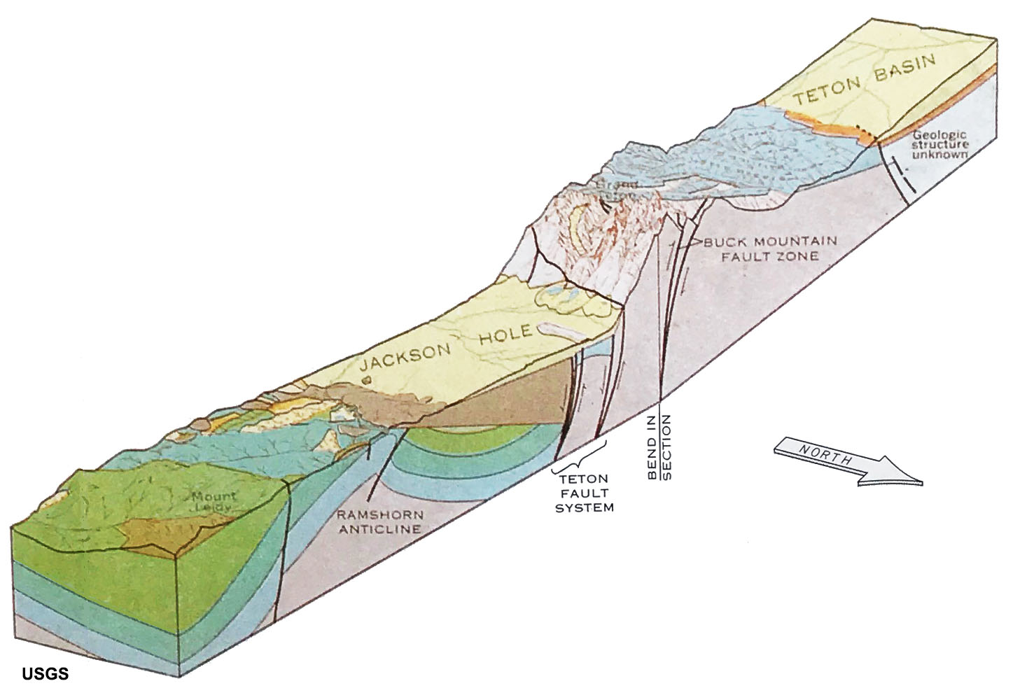
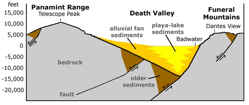
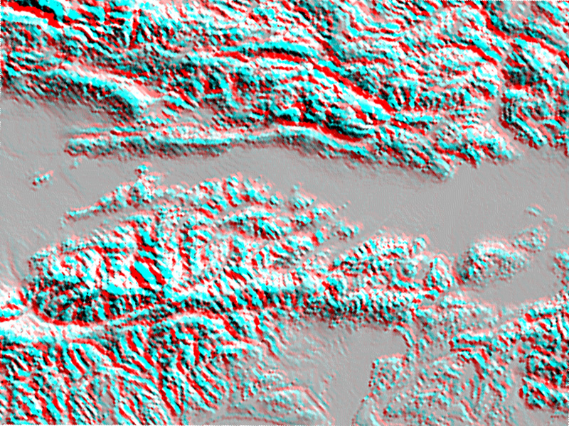
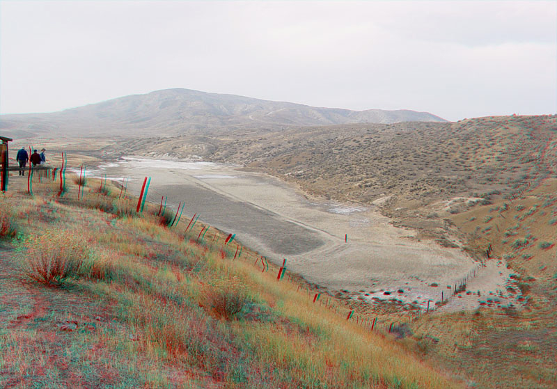
Landscape Features Associated With High-Angle Faults

Seismically active high-angle normal faults are numerous in the western United States, particularly in the Great Basin and surrounding regions (Nevada, Utah, Idaho, Arizona, and eastern California). The Great Basin is undergoing crustal extension on a large scale (see Figure 6-30). Crustal extension is creating massive block-faulted mountain ranges that generally run north-south across the region. Massive normal faults run along many mountain fronts. Many of these range-front faults are considered earthquake faults. Their relatively young geologic age and their ongoing seismic activity results in the steep mountain fronts adjacent to sedimentary filled basins. Range-front faults bordering many of the large mountain ranges are responsible for both dramatic scenery and significant earthquake risks! Examples include: the Wasatch Fault runs along the base of the Wasatch Mountains between Ogden and Salt Lake City, Utah (Figure 6-44); the Owens Valley Fault is responsible for the majestically steep mountain front on the eastern side of the Sierra Nevada Mountains, California (Figure 6-45); Grand Tetons National Park in Wyoming gets its dramatic scenery from the Tetons range-front fault (Figures 6-46 and 6-47); Death Valley is on the eastern side of a range-front fault on the western side of the Funeral Mountains, California (Figures 6-48 and 6-49).

Fig. 6-44. Map of the range-front fault line on the Wasatch Mountains, Ogden, Utah.

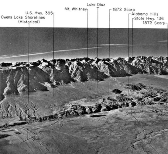Fig. 6-45. Aerial view of the range-front fault in Owens Valley adjacent to the Eastern Sierra Nevada mountain front. The fault produced the Owens Valley Earthquake of 1872 with an estimated magnitude of about 6.8.

Fig. 6-46. The Grand Tetons in Wyoming have risen along great range-front normal fault on the west side of Jackson Hole (basin).

Fig. 6-47. Block diagrams showing the relationship of the Grand Tetons and the Tetons Fault (a range-front normal fault) adjacent to the sediment-filled Jackson Hole basin.

Badwater, the lowest elevation in Death Valley, is located along the range-front fault of the Fueneral Mountains.

Fig. 6-48. Badwater in Death Valley National Park is the lowest elevation in North America (-282 feet). It is adjacent to a range front fault.

Fig. 6-49. Cross section of Death Valley, California illustrating the relationship of the normal fault (the range-front fault near Badwater) on the western side of the Funeral Range and the sediment-filled valley.

6.22

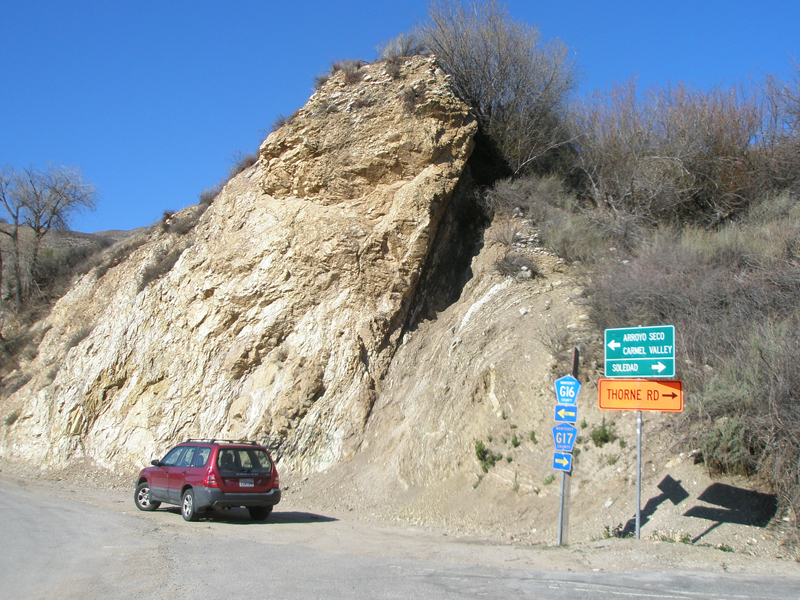
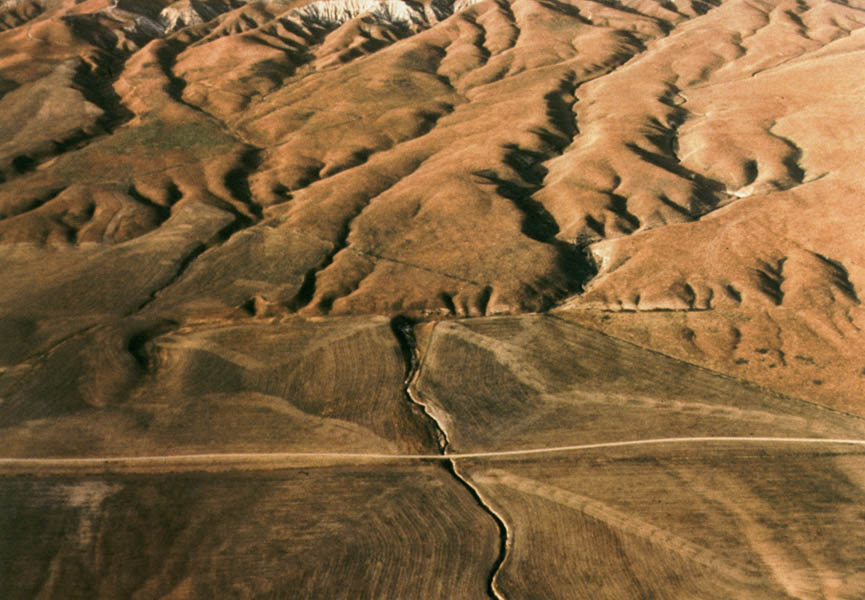
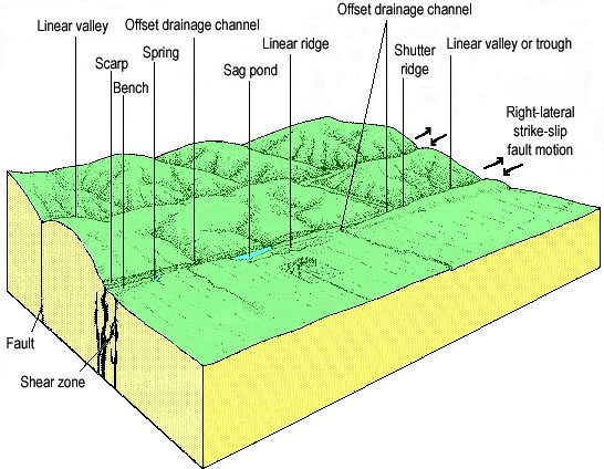
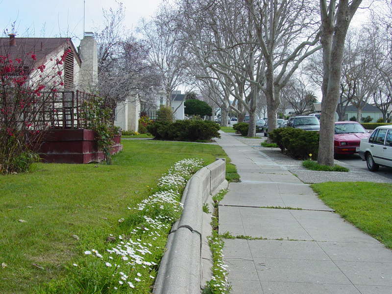
Landscape Features Associated With Strike-Slip Fault Zones (Common in California)

California is famous for its active fault systems, many of the largest faults are strike-slip faults. It is also a dry region, so surface features associated with earthquake fault motion tend to be very well preserved and visible compared to features in wetter climates. Below are examples of landscape features associated with faults that display strike-slip offset (Figure 6-50).

A fault line is the trace of a fault plane intersects the ground surface or other surfaces, such as on a sea cliff, road cut, or in a mine shaft or tunnel. A fault line is the same as fault trace. Faults lines can often be difficult to resolve from general surface observation due to cover by younger sediments, vegetation, and human-induced landscape modifications. They may be revealed by a color change in the soil, but other means are necessary to be sure it is a fault (geologists often dig trenches to study faults). Fault lines are commonly associated with linear features on landscapes, but not all linear features are associated with faults.

An escarpment is a long, more or less continuous cliff or relatively steep slope facing in one general direction, separating two level or gently sloping surfaces. Escarpments are produced both by faulting offset or by erosion of cliff-forming rock bodies along river valleys.

A fault scarp is an escarpment or cliff formed by a fault that reaches the Earth’s surface. Fault scarps tend to be modified by erosion after the faulting occurred (example: Figure 6-51).

A sag pond is a natural depression associated with a fault or associated with a pull-apart basin along a fault system can hold water, even temporarily (example: Figure 6-52).

A linear drainage is a stream drainage that follows the trace of a fault. Stream alignment may be a result of strike-slip fault motion. Streams tend to follow fault zones because the sheared and pulverized rock tend to be easily eroded compared to the surrounding solid bedrock.

A shutter ridge is a ridge formed by vertical, lateral, or oblique displacement on a fault that crosses an area having ridge and valley topography; the displaced part of the ridge shuts in the valley. Shutter ridges typically are found in association with offset drainages (Figure 6-53).

A linear ridge is a long hill or crest of land that stretches in a straight line. It may indicate the presence of a fault or a fold (such as an anticline or syncline). If it is found along a strike-slip fault it may be a shutter ridge or a pressure ridge (example: Figures 6-53 and 6-54).

A linear scarp is a straight escarpment where there is a vertical component of offset along a fault (either normal or reverse). Linear scarps may also form when preferential erosion removes softer bedrock or soil along one side of a fault.

A linear trough is a straight valley that may be bounded by linear fault scarps. A linear trough may be a graben or a rift valley and may be modified by erosion (example: Figure 6-53). Linear troughs are commonly graben-like features and are often called pull-apart basins where they occur in large fault zones (example: Figure 6-54).

An offset drainage is a stream that displays offset by relatively recent movement along a strike-slip fault. A better term is deflected drainage. (example: Figure 6-55).

A side-hill benches is a step-like surface on the side of a hill or mountain. Both recent fault activity or erosional differences of bedrock lithology across a fault may produce side-hill benches and associated linear scarps. Side-hill benches may also form from slumping that may or may not be associated with faulting.

Offset historic infrastructure reveals the location of major faults that are slowly creeping. Offset old fences, broken sidewalks and walls, cracks in old cement and asphalt are common along some of the creeping faults in central California; examples in Figures 6-56 and 6-57.

Fig. 6-50. Geomorphic features associated with strike-slip faults in California (USGS)

Fig. 6-51. Fault scarp on San Andreas Fault in San Juan Bautista, California (left side of trail has risen)

Sag pond along San Andreas Fault on Anzar Road, San Juan Bautista, CA

Fig. 6-52. Sag pond along the San Andreas Fault on Anzar Road, San Juan Bautista, California

3D landscape of the Gilroy, California area

Fig. 6-53. Linear troughs, linear ridges, and shutter ridges associated with faults in the Gilroy and Morgan Hill area, California

Fig. 6-54. Pull-apart basin along the San Andreas Fault, Carrizo Plain National Monument, CA

Fig. 6-55. Offset drainage at Wallace Creek, Carrizo Plain National Monument, CA

Fig. 6-56. Offset wall and sidewalk caused by fault creep on the Calaveras Fault in Hollister, CA

Fig. 6-56. Offset 100 year old culvert caused by fault creep on the San Andreas Fault, DeRose Winery, CA

6.23

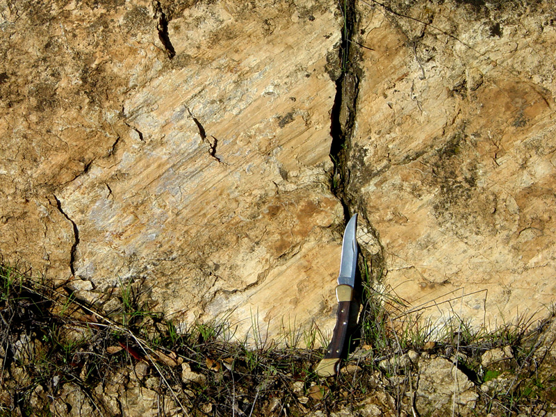
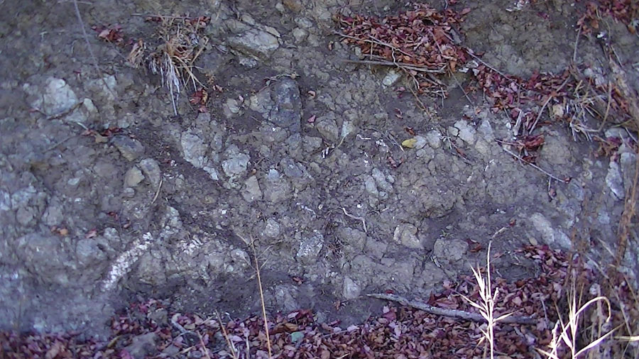
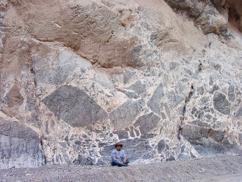
Expressions of Fault Movement On Rocks In Fault Zones

Fault motion fractures, pulverizes, and crushes rock into fragments and powder. Fault zones may be filled with crushed and broken rock through a wide area where large amounts of fault slip have taken place over millions of years. Where exposed by erosion or in cuts associated with construction, material impacted by crushing and shearing fault motion has distinct characteristics:

Slickensides are a polished and striated (scratched) rock surfaces produced by friction along a fault; they appear a scratches on a rock surface (example: Figure 6-58).

Fault gouge is the mix of rock fragments and ground-up rock material in an fault zone; typically uncemented in active fault zones (example: Figure 6-59).

Mylonite is a fine-grained metamorphic rock, typically layered or banded, resulting from the grinding or crushing of other rocks (example: Figure 6-60).

Fault breccia is a mix broken rock fragments (angular grains to massive blocks and boulders) found in a broad fault zone (example: Figure 6-61).

Fig. 6-58. slickensides along the Calaveras Fault, Coyote Lake, Gilroy, California

Fig. 6-59. fault gouge (rock fragments and powder) in the San Andreas Fault Zone, San Benito County, CA

Fig. 6-60. mylonite
ancient fault zone
Southern California

Fig. 6-61. breccia
Titus Canyon, Death Valley, California

6.24

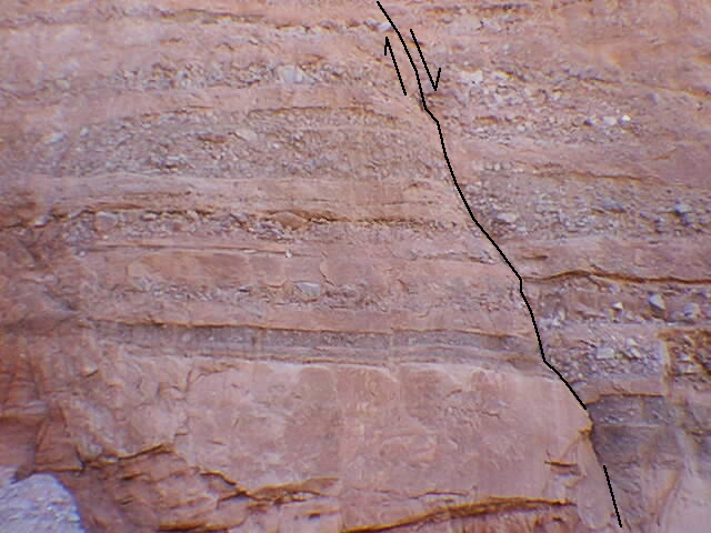
Finding And Interpreting Faults

Trenches are often dug across fault zones to study how earthquakes have offset layers of sediment. Figure 6-62 is an example of a trench profile recorded from a fault zone. Trench studies are conducted to possibly determine the frequency, intensity, and distributions of earthquakes in active fault zones over time, sometimes going back hundreds to thousands of years. Trench studies can often reveal information about the frequency and possible intensity of earthquakes in the geologic past (including in prehistory—before records were kept about earthquake information and recorded, and before seismology became science about 100 years ago).

Geologists use relative and absolute dating methods to try to interpret the earthquake history of faults. After a ground rupturing earthquake, sediment may be deposited over or adjacent to the rupture. Those sediments may contain organic matter that can be dated by radiocarbon dating (C¹⁴/C¹²) methods or other means. Data collected from trenches often reveal potential information about how often earthquake have occurred and sometime the intensity of past earthquakes. In young sediments, the offset caused by earthquakes may be correlated to known strong earthquake in a region. Data from both historic and prehistoric earthquakes can help determine how frequently earthquakes occur, and can be used to estimate when a future earthquake might happen, and the average frequency and intensity of past earthquakes. This information is used to predict earthquake risks and is an important component in earthquake hazard mitigation.

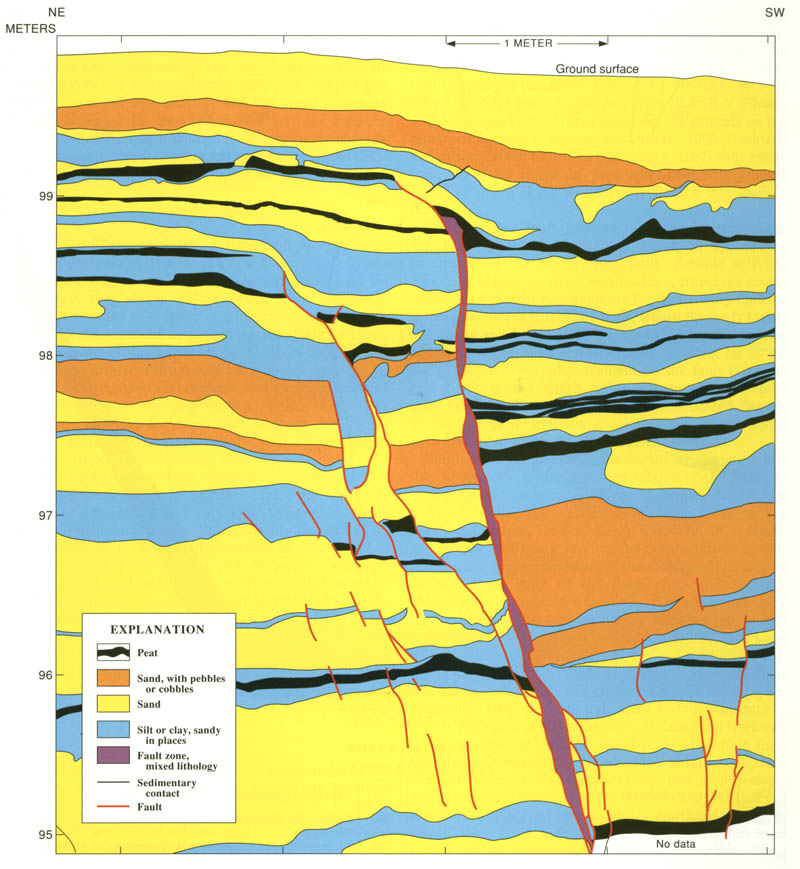Fig. 6-62. Profile of layers of sediments exposed in a trench dug through a young fault.

6.25

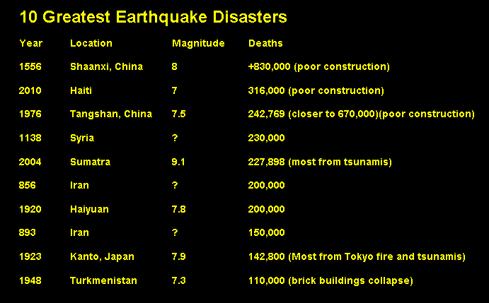
Notable Disasters Associated With Earthquakes And Tsunamis

Earthquakes have been the cause of many great disasters throughout history. Figure 6-62 is a list of the top 10 deadliest or most costly earthquakes. Earthquakes my be the cause of a disaster, but it is often fire, tsunamis, floods, or volcanic eruptions that may contribute to the death and destruction.

Fig. 6-63. Greatest earthquake disasters

Fig. 6-64. Damage from the 1964 Alaska earthquake

Fig. 6-65. Aerial view of the 2010 earthquake in Haiti

Fig. 6-66. Aerial view of San Francisco after the 1906 earthquake and fire

6.26

What Causes Tsunamis?

A tsunami is a very long and/or high sea wave or coastal surge of water caused by an earthquake or other disturbance.

Tsunamis are caused by displacement of the bedrock (seafloor) under an ocean or body of water of any size. They can be generated by earthquakes, volcanic explosions, or underwater landslides. When the solid earth moves, the water above it also moves with it. Tsunamis are the result of both the initial shock waves and the following motion of the water readjusting to a stable pool (sea level). Tsunamis can travel great distances throughout the world's ocean. Their energy is dissipated when they approach shorelines where they come onshore as a great surge of water, with or without a massive waves crashing onshore (Figure 6-6-). Although most tsunamis are small (barely detectable), some modern tsunamis have reached inland elevations many hundreds of feet above sea level. (Tsunamis are discussed in more detail in Chapter 16.)

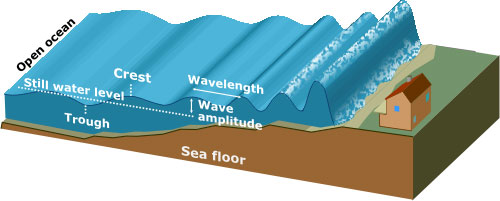Fig. 6-66. How tsunami waves form by fault displacement on the seafloor. Tsunamis can be caused by undersea earthquakes, volcanic eruptions, landslides, or impacts or explosions of any large size.

6.27

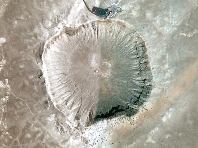
Explosive Impact Structures

Impacts by near Earth asteroids (NEAs) of any size are exceedingly rare, from the 5-megaton limit of atmospheric shielding up to the hundreds of millions of megatons associated with mass extinctions. Statistically, no impact is to be expected within a human lifetime. (Let's hope that is true for ours!)
"The most common estimate has been that the Earth is hit by a civilization threatening impact (by a 1.5-km-diameter asteroid) about twice per million years, which is equivalent to a 1-in-5000 chance per century." --from Asteroid and Comet Impact Hazards: NASA - http://impact.arc.nasa.gov/index.cfm).

Fig. 6-68. Earth's Moon is covered with impact craters; most occurred early in the history of the formation of the Solar System. Earth loses its impact craters through erosion and plate tectonics recycling of the crust.

Fig. 6-69. Meteor Crater, a 50,000 year old, mile wide impact crater near Flagstaff, Arizona (Google satellite view)

Fig. 6-70. Upheaval Dome near Moab, Utah is thought to have an impact origin. It is also thought to be a salt dome (pushed up in the center by salt flowing under pressure at depth).
(Google satellite view)

Impact of the Late Cretaceous in North America

Fig. 6-71. Late Cretaceous impacts in the North America region are thought to have been responsible for the extinction of the dinosaurs and many other life forms.

6.28

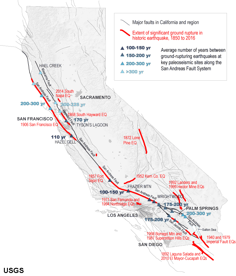
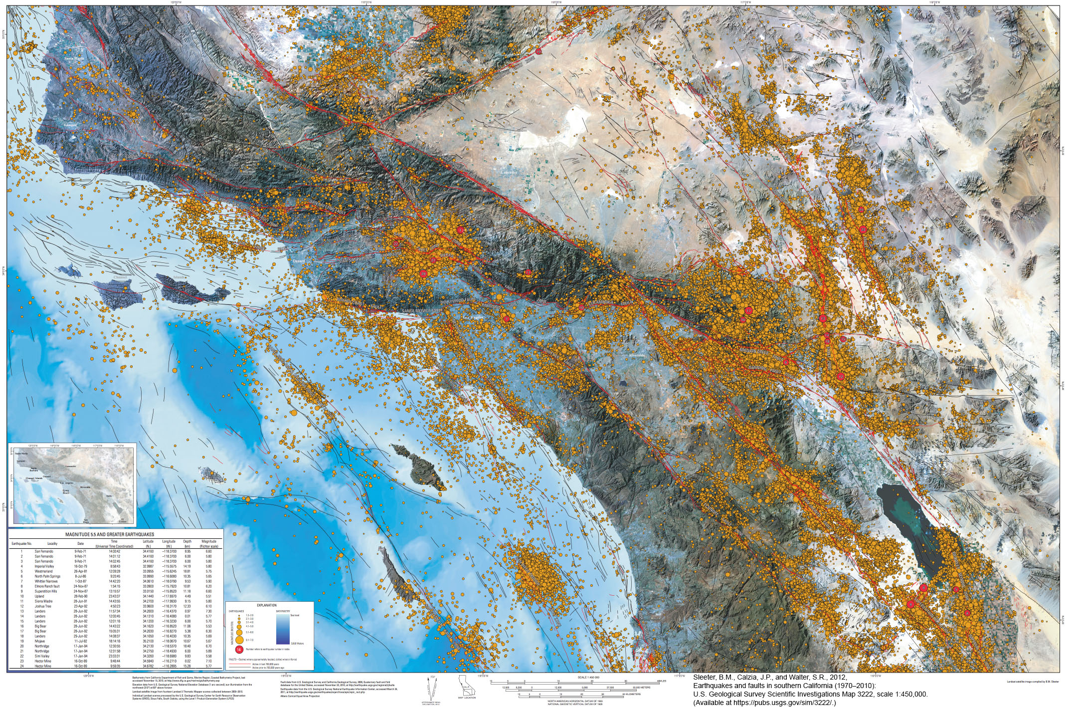
Faults, Earthquake Faults, and Earthquakes in SoCal (Southern California)

Southern California is a very geologically active region. The maps below are very useful for understanding the nature of earthquake hazards in the region. Figure 6-72 shows the location of major historic earthquakes including regions where the major fault displayed surface ruptures and the number of years between major ground-rupturing events where they've been studied in important locations.

Figure 6-73 is a map showing SoCal's regional seismic activity as illustrated with the location of earthquake data recorded between the years of 1970 to 2010. It is interesting to study this map to see which faults, or fault systems were most active within this time window. Faults that do not show a lot of seismic activity on this map may indicate three possible scenarios: 1) the fault is no longer active, 2) the fault already experience an earthquake, and has released most of its stored up energy before 1970, or 3) the fault is locked up and is potentially going to possibly create a major earthquake in the future. It is interesting to study the landscape geography (both topography and bathymetry) relative to the location of the faults on this map. In most cases, the faults are associated with a mountain front (both on land and offshore).

Figure 6-74 shows a map of some of the major earthquake faults in Southern California, displaying characteristics of the faults below the surface. Faults shown as narrow lines are have a vertical orientation, whereas the wider lines show that the faults penetrate into the crust at a low angle (thrust faults). Many of the fault show a component of both horizontal or vertical segments. Almost all the faults are interconnected with other faults in the region. These maps show that the potential for major earthquake may occur both on land or offshore. The ones located offshore could possibly generate massive tsunamis along the SoCal coastline.

Fig. 7-62. Map showing the location of California's major historic earthquakes including those that displayed significant ground rupture (before 2016).

Fig. 6-73. Map showing the location of major faults and the epicenters of earthquakes (1970 to 2010) in Southern California. The base map of this image displays the rugged nature of the landscape associated with this fault zones as well as the bathymetry of the borderlands associated with islands offshore.

Map of low-angle (thrust) and high angle faults in Southern California.

Fig. 6-74. Map showing the detail of many of the faults in Southern California. The width of the color-shaded areas of the different faults shows the general angle that these earthquake faults descend into the crust. Vertical fault are narrow lines, whereas low-angle thrust faults are wider. Some faults show both low-angle and vertical components in different segments of the faults.

6.29

Selected Online Resources About Faults and Earthquakes

The Science of Earthquakes

Faults, Earthquakes, and Landscapes

See: http://earthquake.usgs.gov - The gateway to everything earthquake related at the US Geological Survey.

20 Largest Earthquakes in the World (USGS)

Where is the San Andreas Fault? A Guidebook to Tracing the Fault on Public Lands in the San Francisco Bay Region
This guidebook provides an overview about Bay Area earthquakes and geology.

Where's the Hayward Fault? A Green Guide to the Fault
This guidebook describes the urban geology of the Hayward Fault in the East Bay region.

Putting Down Roots in Earthquake Country
This report includes detail on the "Seven Steps" for earthquake preparedness

Life of a Tsunami (USGS)

Home Safety: Earthquake Preparedness
http://www.homeinsurance.org/home-earthquake-preparedness/

FAQs - Earthquake Preparedness
http://earthquake.usgs.gov/learn/faq/?categoryID=14

6.30

Selected Earthquake Fault Information and Scenarios In California

San Diego Earthquake Planning Scenario, Magnitude 6.9 of the Rose Canyon Fault Zone, Executive Summary
Earthquake Engineerin Research Instutude, San Diego Chapter
Animation of the Scenario M6.9 Earthquake on the Rose Canyon Fault (USGS/SCEC)

Southern California Earthquake Simulation 2016 - M7.8
A simulation of the most likely scenario and effects for the next big earthquake in Southern California.
ShakeOut Scenario - Los Angeles, Detailed Perspective

Computer Simulation of an Earthquake | California Academy of Sciences
A simulation of a potentially large earthquake on the Hayward Fault in the San Francisco Bay Region.

Quiz Questions

https://gotbooks.miracosta.edu/geology/chapter6.html

10/15/2019